Markdown styling in R plots and tables

Of late I have felt very little interest in writing. There are reasons for this, most of which have to do with the rising tide of fascism that seems not to be of much concern to most people in the tech industry, but I personally find a little unsettling since I happen to belong to one of those inconvenient minority groups that fascists love to toss into camps. I am, understandably, preoccupied with that rather than sharing package releases and other things I used to care more about. In all honesty this post is no exception. I just happened to have most of it written months ago and wanted to close the PR. It’s not very interesting, and I don’t really care if you read it.

Anyway, it’s about using markdown syntax in R plots and tables. Whatever. It’s 2026 and the world outside is on fire. Go ask Claude to write your own post if you care about such things. I’m finding it hard to do so anymore.

library(tidyverse)
library(commonmark)
library(conflicted)
library(flextable)
library(ftExtra)
library(ggtext)
library(table1)
library(gt)

conflict_prefer("filter", "dplyr")
conflict_prefer("select", "dplyr")
conflict_prefer("compose", "flextable")

Preface: Labelled data

There is now a well-established – albeit informal – convention in R of using the “label” attribute as a way of storing natural language descriptions of variables,¹ one that is supported by many packages for visualisation such as ggplot2 and some tabulation packages like table1. I’m not entirely sure of the history behind this convention, but from what I can tell it seems to have emerged from the haven and labelled packages, which provide valuable tools built using this idea.

For the purposes of this post I’ll keep it simple, and define some simple helper functions that make it easy to set, get and modify the labels associated with a data set

# get and set the label attribute for a variable
get_label <- function(x) attr(x, "label")
set_label <- function(x, label) {attr(x, "label") <- label; x}

# modify the label attribute of a variable using regular expressions
modify_label <- function(x, pattern, replacement) {
  get_label(x) |> 
    str_replace_all(pattern, replacement) |> 
    set_label(x, label = _)
}

# extract the labels from all variables in a data frame
extract_labels <- function(data) {
  data |> 
    imap(\(x, n) { tibble(
      variable = n, 
      label = get_label(x) %||% NA_character_
    )}) |> 
    list_rbind()
}

# variation of pivot_longer that captures labels rather than variable names
pivot_labels_longer <- function(data, cols, ..., 
                                labels_to = "label", 
                                names_to = "name", 
                                values_to = "value") {
  tbl <- extract_labels(data)
  data |> 
    pivot_longer(
      {{cols}}, 
      ..., 
      names_to = names_to, 
      values_to = values_to
    ) |> 
    mutate(
      {{labels_to}} := .data[[names_to]] |> 
        recode_values(
          from = tbl$variable, 
          to = tbl$label
        )
    )
}

These functions are all written on the assumption that tidyverse packages are loaded (specifically dplyr, tidyr, purrr, stringr, and tibble), and they won’t work with older versions of R that don’t support the base pipe, anonymous function syntax, or null coalescing operator, but it would not be difficult to express the same idea in base R or with older R versions. Moreover, these functions alone make for a very limited toolkit for working with variable labels, but they will be good enough for what I need in this post.

Having done so, I’ll now need some data to use as an example. To that end I simulated a simple exposure-response data set, similar to the kind of data that arise in pharmacometric analyses, though quite a bit simpler than a real world data set would be. I’ll import the data now, and supply variable labels that we might want to use in figures and tables.

dat <- read_csv("er.csv", show_col_types = FALSE) |> 
  mutate(
    id   = factor(id),
    sex  = factor(sex),
    dose = factor(dose)
  ) |> 
  mutate(
    id       = id       |> set_label("Subject Identifier"),
    dose     = dose     |> set_label("Dose (mg/m^2)"),
    aucss    = aucss    |> set_label("AUCss (ng.h/mL)"),
    cmaxss   = cmaxss   |> set_label("Cmax,ss (ng/mL)"),
    response = response |> set_label("Response (units)"),
    ae       = ae       |> set_label("Adverse Event"),
    sex      = sex      |> set_label("Sex"),
    age      = age      |> set_label("Age (years)"),
    weight   = weight   |> set_label("Weight (kg)"),
    height   = height   |> set_label("Height (cm)"),
    bsa      = bsa      |> set_label("Body Surface Area (m^2)")
  )

dat

# A tibble: 300 × 11
   id    dose   aucss cmaxss response    ae sex      age weight height   bsa
   <fct> <fct>  <dbl>  <dbl>    <dbl> <dbl> <fct>  <dbl>  <dbl>  <dbl> <dbl>
 1 1     30    10884.  1161.     15.6     1 Male      51   98.4    175  2.14
 2 2     10     7952.   734.     12.8     0 Male      31   77      164  1.83
 3 3     20     9466.  1104.     11.9     0 Female    29   60.8    162  1.64
 4 4     30    32578.  3061.     18.1     1 Male      51   99.5    183  2.21
 5 5     20    12504.  1050      14.0     1 Female    25   67.3    154  1.65
 6 6     10     4851.   468.     12.1     1 Male      38   60.9    150  1.56
 7 7     20    10902.  1290.     13.5     1 Female    33   52.1    163  1.55
 8 8     30    15205.  1386      16.4     1 Male      45  116.     174  2.28
 9 9     20     7596.  1367.     14.9     1 Male      48   93.1    184  2.16
10 10    30    21906.  1893.     14.4     1 Female    26  110.     164  2.13
# ℹ 290 more rows

Although the labels don’t appear in this output, they are stored internally:

extract_labels(dat)

# A tibble: 11 × 2
   variable label                  
   <chr>    <chr>                  
 1 id       Subject Identifier     
 2 dose     Dose (mg/m^2)          
 3 aucss    AUCss (ng.h/mL)        
 4 cmaxss   Cmax,ss (ng/mL)        
 5 response Response (units)       
 6 ae       Adverse Event          
 7 sex      Sex                    
 8 age      Age (years)            
 9 weight   Weight (kg)            
10 height   Height (cm)            
11 bsa      Body Surface Area (m^2)

Conveniently, more recent versions of ggplot2 will respect these labels and use them in plots if the user doesn’t explicitly specify the labels. If I wanted to draw boxplots of AUCss exposure stratified by sex, I could do so like this and ggplot2 will use the labels I provided earlier:

dat |> 
  ggplot(aes(aucss, sex)) + 
  geom_boxplot()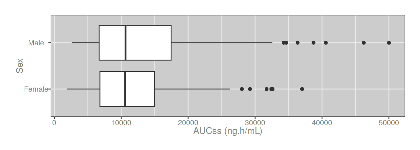

Markdown in ggplot2

Using subscripts is easy

In most cases a boxplot like the one in the previous section is perfectly fine for scientific purposes, but sometimes it’s necessary to be a little more precise. Conventionally the “ss” in “AUCss” is written as a subscript rather than regular lower-case font, so the x-axis label is more accurately written as “AUC_ss”. In this text document I can render the subscripts easily using markdown notation. To do the same thing in a ggplot2 figure is slightly more complicated because ggplot2 does not natively support markdown syntax.² Fortunately, the ggtext package by Claus Wilke exists. To apply subscripts in my x-axis label, all I need to do is add the markdown syntax in the label using the modify_label() function I wrote earlier, and use element_markdown() in the relevant part of the ggplot2 theme:

dat |> 
  mutate(aucss = aucss |> modify_label("AUCss", "AUC<sub>ss</sub>")) |> 
  ggplot(aes(aucss, sex)) + 
  geom_boxplot() + 
  theme(axis.title.x = element_markdown())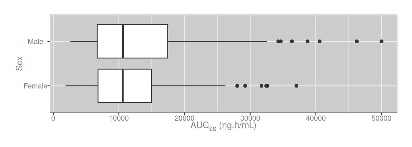

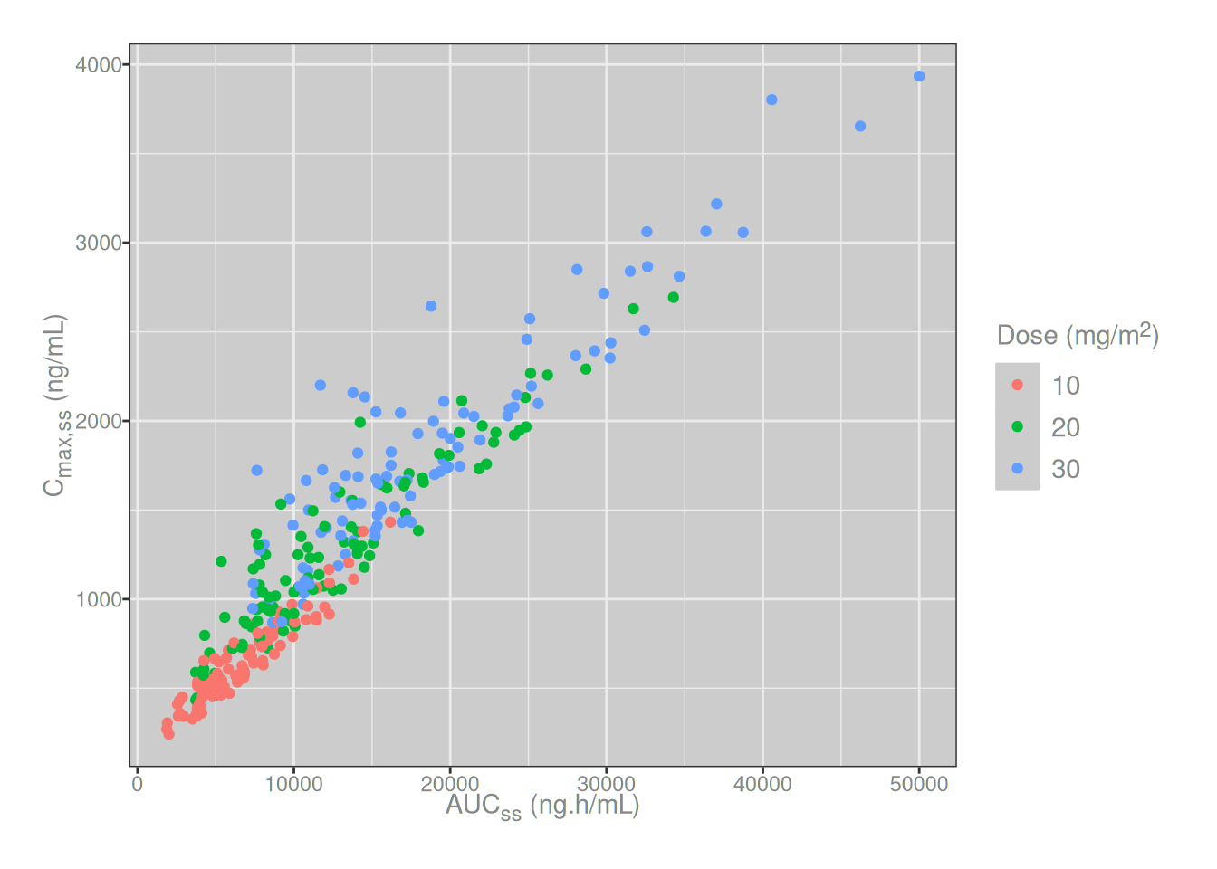
The element_markdown() approach works just as easily when markdown syntax is required in a plot legend instead of (or in addition to) the axis labels. For example, suppose I want to create an exposure correlation plot that shows the relationship between C_max,ss and AUC_ss, with colour used to denote the dosing group for each subject. For this hypothetical drug, the actual dose (in milligrams) is proportional to body surface area (units in m²), so the units for our dose groups should be displayed as mg/m² in the legend. This also is easy:

dat |> 
  mutate(
    aucss  = aucss  |> modify_label("AUCss", "AUC<sub>ss</sub>"),
    cmaxss = cmaxss |> modify_label("Cmax,ss", "C<sub>max,ss</sub>"),
    dose   = dose   |> modify_label("m\\^2", "m<sup>2</sup>") 
  ) |> 
  ggplot(aes(aucss, cmaxss, color = dose)) + 
  geom_point() +
  theme(
    axis.title.x = element_markdown(),
    axis.title.y = element_markdown(),
    legend.title = element_markdown()
  )

Sometimes the plot needs to be faceted, with exposure metric as the faceting variable. In that situation a little bit of data wrangling comes in handy and it it is convenient to use the pivot_labels_longer() function to capture the labels as well as the variable names:

dat_long <- dat |> 
  pivot_labels_longer(
    cols = c(aucss, cmaxss),
    names_to = "metric",
    labels_to = "metric_label",
    values_to = "exposure"
  ) |>
  mutate(
    metric = metric |> set_label("Metric"),
    metric_label = metric_label |> set_label("Metric"),
    exposure = exposure |> set_label("Exposure")
  )

dat_long

# A tibble: 600 × 12
   id    dose  response    ae sex      age weight height   bsa metric
   <fct> <fct>    <dbl> <dbl> <fct>  <dbl>  <dbl>  <dbl> <dbl> <chr> 
 1 1     30        15.6     1 Male      51   98.4    175  2.14 aucss 
 2 1     30        15.6     1 Male      51   98.4    175  2.14 cmaxss
 3 2     10        12.8     0 Male      31   77      164  1.83 aucss 
 4 2     10        12.8     0 Male      31   77      164  1.83 cmaxss
 5 3     20        11.9     0 Female    29   60.8    162  1.64 aucss 
 6 3     20        11.9     0 Female    29   60.8    162  1.64 cmaxss
 7 4     30        18.1     1 Male      51   99.5    183  2.21 aucss 
 8 4     30        18.1     1 Male      51   99.5    183  2.21 cmaxss
 9 5     20        14.0     1 Female    25   67.3    154  1.65 aucss 
10 5     20        14.0     1 Female    25   67.3    154  1.65 cmaxss
# ℹ 590 more rows
# ℹ 2 more variables: exposure <dbl>, metric_label <chr>

Once in that form, we can easily create the desired plot using exposure as the x-axis variable and metric_label as the facetting variable:

dat_long |> 
  ggplot(aes(exposure, sex)) + 
  geom_boxplot() +
  facet_wrap(~metric_label, scale = "free_x")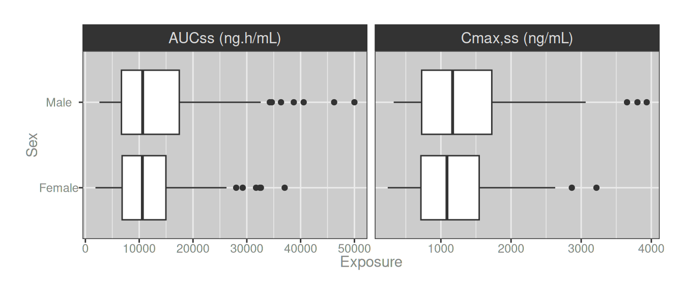

Again, subscript support is easy with element_markdown()

dat_long |> 
  mutate(
    metric_label = metric_label |> 
      str_replace_all("AUCss", "AUC<sub>ss</sub>") |> 
      str_replace_all("Cmax,ss", "C<sub>max,ss</sub>")
  ) |> 
  ggplot(aes(exposure, sex)) + 
  geom_boxplot() +
  facet_wrap(~metric_label, scale = "free_x") +
  theme(strip.text = element_markdown())

Using subscripts with label wrapping is not

Up to this point, all I’ve really done is illustrate basic ggtext functionality, but the nice thing about ggtext is that the basic functionality actually covers the vast majority of things I need to accomplish with markdown inside ggplot2. There are a few exceptions though. One case where you have to be a little more sophisticated is when you need automatic label wrapping for your markdown-formatted text in a plot.

To illustrate the point, let’s imagine a case where I want to create a faceted plot with very long strip text labels. Let’s say that these are moy labels:

long_labels <- c(
  aucss = paste(
    "The term 'AUCss' is used to denote",
    "the area under the concentration-time",
    "curve at steady state"
  ),
  cmaxss = paste(
    "The term 'Cmax,ss' is used to denote",
    "the maximum concentration at steady",
    "state"
  )
)

dat_long <- dat_long |> 
  mutate(
    long_metric_label = metric |> 
      recode_values(
        from = c("aucss", "cmaxss"),
        to = long_labels
      )
  )

If I try to create my faceted boxplot using these labels I get a very ugly output:

dat_long |> 
  ggplot(aes(exposure, sex)) + 
  geom_boxplot() +
  facet_wrap(~long_metric_label, scale = "free_x")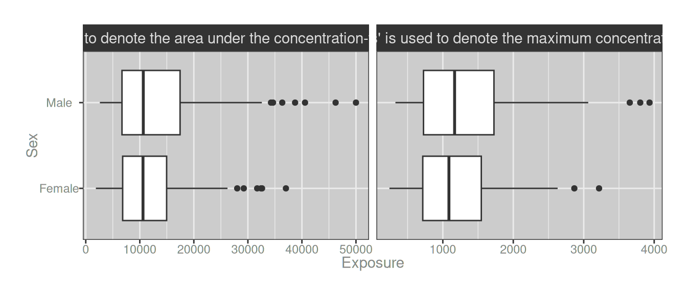

So far my labels don’t use any markdown formatting, but let’s follow it through and consider how we usually solve this problem in ggplot2. The tool I always use in this scenario is ggplot2::label_wrap_gen(), which allows me to define a labeller function that automatically wraps the strip text across multiple lines:

labeller_1 <- label_wrap_gen(28)

dat_long |> 
  ggplot(aes(exposure, sex)) + 
  geom_boxplot() +
  facet_wrap(~long_metric_label, scales = "free_x", labeller = labeller_1)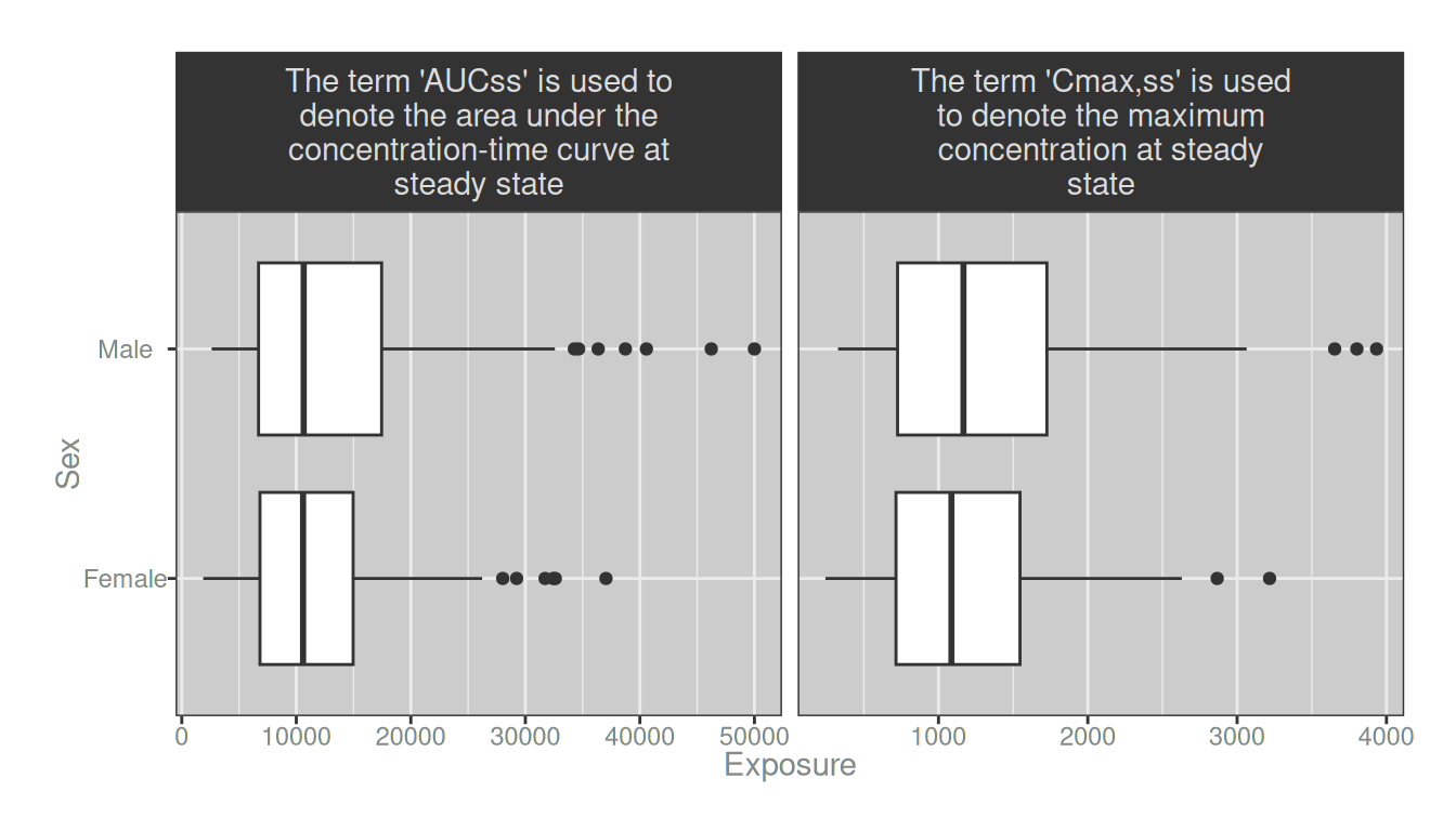

Woohoo! Problem solved.

Well… sort of. The label_wrap_gen() solution works nicely, as long as your strip labels are plain text. It becomes a lot more difficult, however, if you need to apply markdown styling to the strip text. Suppose I want to highlight the names of the two exposure metrics by making the text bold, and use subscripts to be more precise in how they are formatted. Inserting the required markdown formatting is not difficult:

dat_long <- dat_long |> 
  mutate(
    long_metric_label = long_metric_label |> 
      str_replace("'AUCss'", "**AUC<sub>ss</sub>**") |> 
      str_replace("'Cmax,ss'", "**C<sub>max,ss</sub>**")
  )

However, we now have a problem. If I use my labeller function I get wrapped strip labels just like before, but the markdown doesn’t get parsed:

dat_long |> 
  ggplot(aes(exposure, sex)) + 
  geom_boxplot() +
  facet_wrap(~long_metric_label, scales = "free_x", labeller = labeller_1)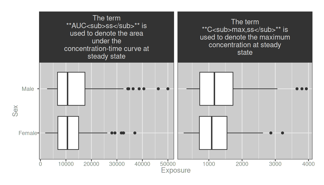

Well yes obviously it doesn’t get parsed because I’m not using ggtext here. But when I try to combind element_markdown() with my labeller function, it prevents the wrapping from working:³

dat_long |> 
  ggplot(aes(exposure, sex)) + 
  geom_boxplot() +
  facet_wrap(~long_metric_label, scales = "free_x", labeller = labeller_1) +
  theme(strip.text = element_markdown())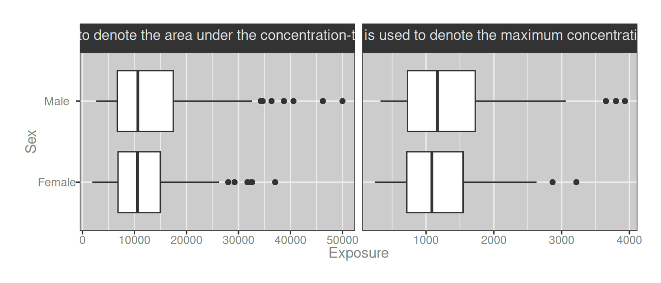

A solution to the problem requires three things:

• We need a label_wrap_gen_md() function that behaves like ggplot2::label_wrap_gen() that works with markdown text rather than regular R strings (i.e., it needs to parse ggplot2 strip labels and automatically insert markdown line breaks). But to do that;
• We need a str_wrap_md() function that behaves like stringr::str_wrap() that works with markdown text rather than regular R strings (i.e., it needs to insert line breaks with "<br>" rather than "\n", and it needs to wrap based on the length of the markdown output text not the lengh of the markdown string itself). But to do that;
• We need a str_length_md() function that behaves like stringr::str_length() that calculates (or approximates) how long a markdown string will be after it has been processed (i.e., ignore non-printing HTML)

In other words, what I need to do is this:

str_length_md <- function(string) string |> 
  map_int(\(x) str_length(markdown_text(x)) - 1L) 

str_wrap_md <- function(string, width = 80, sep = "<br>") {
  accum <- \(acc, x) {
    last <- acc[length(acc)]
    rest <- acc[-length(acc)]
    merge_length <- str_length_md(last) + str_length_md(x)
    if (merge_length > width) return(c(acc, x))
    c(rest, paste(last, x))
  }
  chunks <- map(str_split(string, " "), \(x) reduce(x, accum))
  map_chr(chunks, \(x) paste(x, collapse = sep))
}

label_wrap_gen_md <- function(width = 25, multi_line = TRUE) {
  fn <- \(labels) label_value(labels, multi_line = multi_line) |> 
     map(\(x) str_wrap_md(x, width = width, sep = "<br>"))
  structure(fn, class = "labeller")
}

labeller_2 <- label_wrap_gen_md(28)

dat_long |> 
  ggplot(aes(exposure, sex)) + 
  geom_boxplot() +
  facet_wrap(~long_metric_label, scales = "free_x", labeller = labeller_2) +
  theme(strip.text = element_markdown())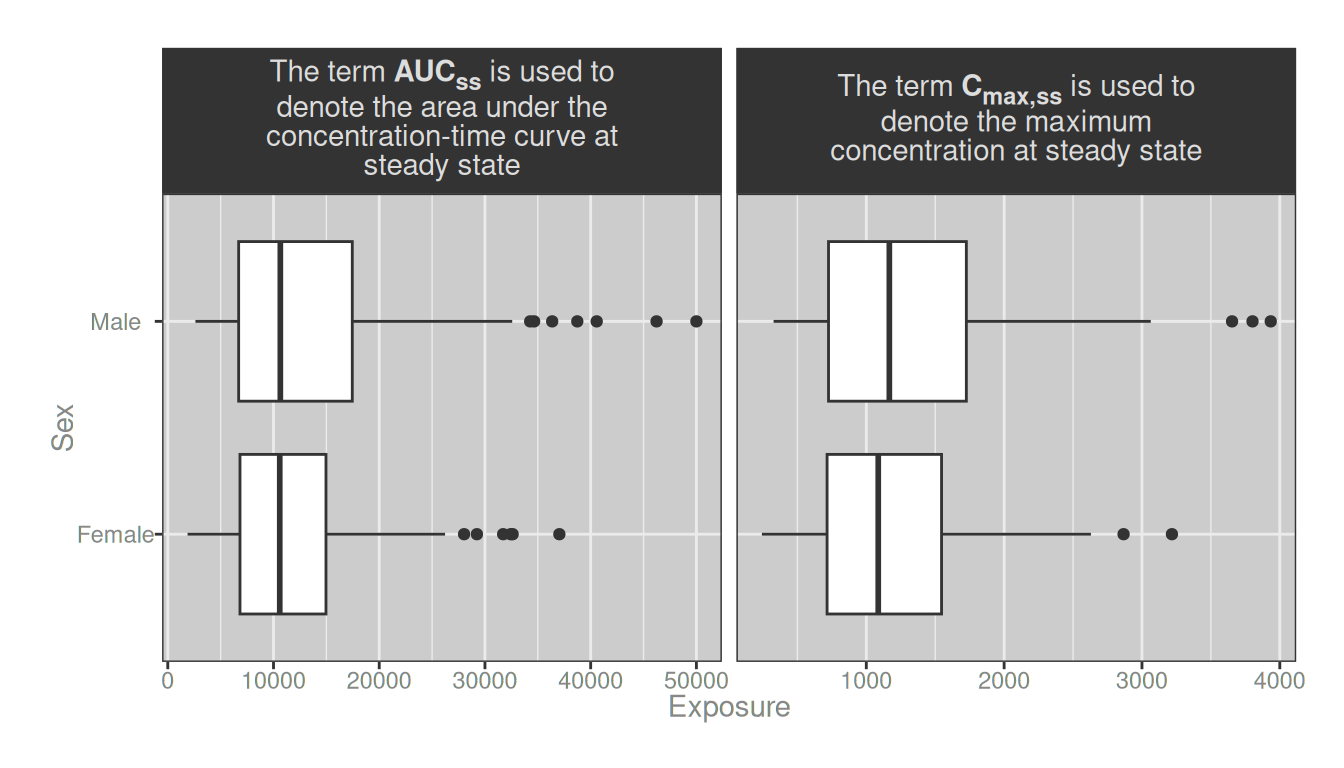

Problem solved! 🎉

How does the trick work?

long_labels_md <- long_labels |>
  str_replace("'AUCss'", "**AUC<sub>ss</sub>**") |> 
  str_replace("'Cmax,ss'", "**C<sub>max,ss</sub>**")

str_wrap(long_labels_md, width = 28)

                                                                                                            aucss 
"The term\n**AUC<sub>ss</sub>** is used\nto denote the area under the\nconcentration-time curve at\nsteady state" 
                                                                                                           cmaxss 
                "The term\n**C<sub>max,ss</sub>** is\nused to denote the maximum\nconcentration at steady\nstate" 

str_wrap_md(long_labels_md, width = 28)

                                                                                                                 aucss 
"The term **AUC<sub>ss</sub>** is used to<br>denote the area under the<br>concentration-time curve at<br>steady state" 
                                                                                                                cmaxss 
                   "The term **C<sub>max,ss</sub>** is used to<br>denote the maximum<br>concentration at steady state" 

To see it a little more clearly, this is how str_wrap() separates the strings:

long_labels_md |> 
  str_wrap(width = 28) |> 
  cat(sep = "\n\n")

The term
**AUC<sub>ss</sub>** is used
to denote the area under the
concentration-time curve at
steady state

The term
**C<sub>max,ss</sub>** is
used to denote the maximum
concentration at steady
state

It looks pretty evenly split, but a lot of space is occupied by the HTML tags that don’t show up when the markdown is rendered. That means that after the markdown is rendered, we end up with something that doesn’t look right:

long_labels_md |> 
  str_wrap(width = 28) |> 
  map_chr(markdown_text) |> 
  cat(sep = "\n\n")

The term
AUCss is used
to denote the area under the
concentration-time curve at
steady state


The term
Cmax,ss is
used to denote the maximum
concentration at steady
state

By contrast, this is how str_wrap_md() wraps the strings,

long_labels_md |> 
  str_wrap_md(width = 28, sep = "\n") |> 
  cat(sep = "\n\n")

The term **AUC<sub>ss</sub>** is used to
denote the area under the
concentration-time curve at
steady state

The term **C<sub>max,ss</sub>** is used to
denote the maximum
concentration at steady state

It looks irregular initially, but once the HTML tags disappear…

long_labels_md |> 
  str_wrap_md(width = 28, sep = "\n") |> 
  map_chr(markdown_text) |> 
  cat(sep = "\n\n")

The term AUCss is used to
denote the area under the
concentration-time curve at
steady state


The term Cmax,ss is used to
denote the maximum
concentration at steady state

…we’re all good.

Markdown in tables

In all honesty, I only really wanted to write the ggplot2 example, because that’s the situation that creates headaches for me most often. But since I was already thinking about markdown in tables, I thought it would be worth writing down a few notes on that as well. I mean why not? It won’t be very interesting, but at least it will be brief. There are three packages I typically use to make tables: table1, gt, and flextable1. Let’s go through them in turn.

With table1

The easiest case to think about is table1, because it works out of the box and there really isn’t anything special you have to do. Since its output is always HTML, HTML markup embedded in variable labels renders directly in the browser. Using the same modify_label() approach as before, I can embed HTML subscripts and superscripts in the relevant labels before passing the data to table1():

dat |> 
  mutate(
    dose   = dose   |> modify_label("m\\^2", "m<sup>2</sup>"),
    aucss  = aucss  |> modify_label("AUCss", "AUC<sub>ss</sub>"),
    cmaxss = cmaxss |> modify_label("Cmax,ss", "C<sub>max,ss</sub>"),
    bsa    = bsa    |> modify_label("m\\^2", "m<sup>2</sup>")
  ) |>
  table1(~ sex + age + weight + height + bsa | dose, data = _)

	10 (N=100)	20 (N=100)	30 (N=100)	Overall (N=300)
Sex
Female	54 (54.0%)	48 (48.0%)	41 (41.0%)	143 (47.7%)
Male	46 (46.0%)	52 (52.0%)	59 (59.0%)	157 (52.3%)
Age (years)
Mean (SD)	39.8 (9.43)	39.6 (9.12)	42.4 (8.79)	40.6 (9.17)
Median [Min, Max]	38.5 [22.0, 58.0]	39.0 [23.0, 59.0]	43.5 [22.0, 59.0]	40.0 [22.0, 59.0]
Weight (kg)
Mean (SD)	86.0 (24.9)	84.1 (22.1)	85.2 (23.3)	85.1 (23.4)
Median [Min, Max]	80.4 [46.4, 170]	80.9 [49.6, 144]	80.1 [43.1, 160]	80.3 [43.1, 170]
Height (cm)
Mean (SD)	168 (10.8)	169 (10.2)	169 (10.1)	169 (10.4)
Median [Min, Max]	168 [140, 193]	169 [148, 188]	169 [145, 195]	168 [140, 195]
Body Surface Area (m2)
Mean (SD)	1.95 (0.298)	1.93 (0.258)	1.95 (0.271)	1.94 (0.276)
Median [Min, Max]	1.92 [1.42, 2.89]	1.95 [1.48, 2.46]	1.92 [1.39, 2.78]	1.94 [1.39, 2.89]

The subscripts and superscripts in the row labels render correctly without anything analogous to element_markdown(). That effortlessness is a direct consequence of table1 only ever producing HTML output. There’s is no rendering problem to solve. Easy.

With gt

Moving on.

In the table1 example above, the data summaries and the rendering are both handled by the table1() function. That’s not how it works with either gt or flextable, which separate the data summarisation and the rendering into two distinct steps. In both cases, the data is summarised first, and then the table is rendered in a second step. So I’ll start by creating a simple data summary table showing mean and standard deviations for each exposure metric, stratified by dose group, using sprintf() to combine the values into a single string for each metric:

dat_smm <- dat |>
  summarise(
    n        = n(),
    aucss    = sprintf("%.0f (%.0f)", mean(aucss), sd(aucss)),
    cmaxss   = sprintf("%.0f (%.0f)", mean(cmaxss), sd(cmaxss)),
    response = sprintf("%.2f (%.2f)", mean(response), sd(response)),
    .by = dose,
  ) 

dat_smm

# A tibble: 3 × 5
  dose      n aucss        cmaxss     response    
  <fct> <int> <chr>        <chr>      <chr>       
1 30      100 18642 (8850) 1848 (641) 15.73 (1.42)
2 10      100 6682 (3008)  646 (235)  13.44 (1.83)
3 20      100 12696 (6679) 1277 (489) 14.70 (1.53)

Truly thrilling.

Okay, now we make the table. Again, gt and flextable differ from table1 in an important way. They are format-agnostic: they can produce output in multiple formats, not just HTML, so we need to do a little more work to tell the packages how to handle the formatting information. The gt package has an explicit system for rich text content supported via wrapper functions like html() and md() that tell it how to interpret column labels. For subscripts and superscripts, html() will work fine:

dat_smm |>
  gt() |>
  cols_label(
    dose     = html("Dose (mg/m<sup>2</sup>)"),
    n        = "N",
    aucss    = html("AUC<sub>ss</sub> (ng·h/mL)"),
    cmaxss   = html("C<sub>max,ss</sub> (ng/mL)"),
    response = "Response (units)"
  ) |>
  tab_footnote("Values are mean (SD).")

Dose (mg/m2)	N	AUCss (ng·h/mL)	Cmax,ss (ng/mL)	Response (units)
30	100	18642 (8850)	1848 (641)	15.73 (1.42)
10	100	6682 (3008)	646 (235)	13.44 (1.83)
20	100	12696 (6679)	1277 (489)	14.70 (1.53)
Values are mean (SD).

You could also use md() in the same position if you want, though standard markdown has no subscript syntax so it doesn’t buy us much. In this instance you’d still need to fall back on HTML tags inside the md() string anyway.

In any case, it’s pretty clear that you don’t have to work very hard to get subscripts and superscripts to render correctly in gt tables. The only thing you have to do is wrap the relevant column labels in html() or md(), and the rest is handled automatically.

With flextable

The only case left to consider is flextable. On the surface, it would seem like it’s an enormous pain to support subscripts and/or markdown syntax within the package. The native approach to rich text within flextable is compositional rather than markup-based: instead of writing "AUC<sub>ss</sub>" as a string, you assemble the label from pieces using as_paragraph(), as_sub(), and as_sup(). So your code is kind of annoying:

dat_smm |> 
  flextable() |>
  compose(
    part = "header", j = "dose",
    value = as_paragraph("Dose (mg/m", as_sup("2"), ")")
  ) |>
  compose(
    part = "header", j = "n",
    value = as_paragraph("N")
  ) |>
  compose(
    part = "header", j = "aucss",
    value = as_paragraph("AUC", as_sub("ss"), " (ng·h/mL)")
  ) |>
  compose(
    part = "header", j = "cmaxss",
    value = as_paragraph("C", as_sub("max,ss"), " (ng/mL)")
  ) |>
  compose(
    part = "header", j = "response",
    value = as_paragraph("Response (units)")
  ) |>
  add_footer_lines("Values are mean (SD).") |>
  bg(bg = "white", part = "all") |>
  autofit()

Dose (mg/m2)	N	AUCss (ng·h/mL)	Cmax,ss (ng/mL)	Response (units)
30	100	18642 (8850)	1848 (641)	15.73 (1.42)
10	100	6682 (3008)	646 (235)	13.44 (1.83)
20	100	12696 (6679)	1277 (489)	14.70 (1.53)
Values are mean (SD).

Thankfully there is an easy workaround if you happen to be a human being rather than a machine and would prefer semi-readable markdown rather than the monstrosity in the previous code snippet. Specifically, the ftExtra package by Atsushi Yamamoto provides colformat_md(), which runs pandoc over the cell content and converts it to flextable’s native rich text. Pandoc markdown uses ^text^ for superscripts and ~text~ for subscripts, which is super convenient because now our table code looks like this:

dat_smm |>
  flextable() |>
  set_header_labels(
    dose     = "Dose (mg/m^2^)",
    n        = "N",
    aucss    = "AUC~ss~ (ng·h/mL)",
    cmaxss   = "C~max,ss~ (ng/mL)",
    response = "Response (units)"
  ) |>
  colformat_md(part = "header") |>
  add_footer_lines("Values are mean (SD).") |>
  bg(bg = "white", part = "all") |>
  autofit()

Dose (mg/m2)	N	AUCss (ng·h/mL)	Cmax,ss (ng/mL)	Response (units)
30	100	18642 (8850)	1848 (641)	15.73 (1.42)
10	100	6682 (3008)	646 (235)	13.44 (1.83)
20	100	12696 (6679)	1277 (489)	14.70 (1.53)
Values are mean (SD).

The result is identical, but the intent is much easier to read. colformat_md() can also be applied to the body of the table, not just the header, which makes it useful any time cell values themselves contain markdown-formatted text. Not super complicated once you know the trick, but as usual in life nobody ever bothers to tell you the trick until after you’ve wasted hours of your life writing the ugliest code known to humankind.

Oh well.

Footnotes

1. More precisely, the “label” attribute is used to store variable labels. Value labels are often stored in the “labels” attribute, allowing natural conversion to factors where the same information becomes the “levels” attribute

2. More traditionally you can pass an R expression that can be handled via ggplot2::label_parse(), but (a) the syntax sucks, and (b) it turns out that when try to solve the hard problem later on, the expression syntax is even more of a pain to work with than markdown

3. This is because the labeller uses "\n" to insert line breaks, but markdown requires us to use "<br>"