Linear cosine palettes

So. Looking back at my history on this blog I have noticed that I, ummmmmm, tend to write long posts. It is a character flaw of which I am acutely aware. When I want to understand a thing I feel a kind of psychological compulsion to delve too deeply into the darkness, dive into to as many of the specifics as I possibly can, organise my thoughts around those specifics, and then drag the whole cursed mess into the daylight so that my long-suffering readers can look on in horror at the grotesquerie of my inner world.

I am aware that this is perhaps unwise.

Reflecting on this as a personal weakness, I have set myself a challenge this fine Sunday: is it even possible for me to write a simple blog post? Like, is it even possible for a mediocre bitch to write a short goddamn article without turning it into some macabre monograph? Given my past form, it is not at all obvious that I’m capable of this level of self-restraint. Let’s see if I can do it?

Linear cosine palettes

The motivation came from this mastodon post by Mike Cheng proposing a simple method for randomly generating continuous colour palettes in R. The original idea comes from a blog post by Inigo Quilez on simple procedural palettes, and the idea is painfully simple. Let’s say we have length-3 vectors \(\mathbf{a}\), \(\mathbf{b}\), \(\mathbf{c}\), and \(\mathbf{d}\) representing four “base” colours from which a continous palette is to be generated. In R we could choose these base colours using the colors() function. Once these are selected we can define a smooth palette using the following function

\[ f(t) = \mathbf{a} + \mathbf{b} \ \cos(2 \pi(\mathbf{c} t + \mathbf{d})) \]

where \(t\) is varied from 0 to 1. The nice thing about this paletting rule is that it can be very fast, especially since – I am told by people who understand such things – there are a lot of optimisations in modern CPUs and GPUs to make cosine evaluation fast. Admittedly, speed is not something I care about much in my generative art work because palette generation is not even close to being a bottleneck in my code and also I’m lazy.

Okay, so here’s an R function that implements a very minor tweak on Mike’s implementation of Inigo Quilez’ cosine palettes:

cosine_palette <- function(n, base = NULL, seed = NULL) {
  if (!is.null(seed)) set.seed(seed)
  if (is.null(base)) base <- colors(distinct = TRUE)
  a <- c(0.5, 0.5, 0.5)
  b <- (sample(base, 1) |> col2rgb() |> as.vector()) / 255
  c <- (sample(base, 1) |> col2rgb() |> as.vector()) / 255
  d <- (sample(base, 1) |> col2rgb() |> as.vector()) / 255
  pal <- vapply(
    seq(0, 1, length.out = n), 
    function(t) a + b * cos(2 * pi * (c * t + d)), 
    double(3)
  )
  pal[pal > 1] <- 1
  rgb(t(abs(pal)))
}

cosine_palette(n = 16, seed = 11)

 [1] "#7F1616" "#6F1A17" "#362A20" "#22442F" "#8A6642" "#F18A5A" "#FFAD74"
 [8] "#FFCB8F" "#FFE0A9" "#FFE9C0" "#FFE6D3" "#AAD6E1" "#40BDE8" "#1F9CE9"
[15] "#6377E3" "#7F54D6"

That’s nice, but as my visual cortex is not optimised for the interpretation of hexadecimal RGB colour codes, I find it convenient to show palettes using… check notes… images? Yes. Yes, that sounds right. To that end I’ll use this shade_strip() that I sometimes use to display a continuously varying palette as a strip:

shade_strip <- function(cols) {
  withr::with_par(
    list(mar = c(0,0,0,0)),
    image( matrix(seq_along(cols), ncol = 1), col = cols, axes = FALSE)
  )
}

seeds <- 11:22
seeds |> 
  purrr::map(\(s) cosine_palette(n = 256, seed = s)) |> 
  purrr::walk(shade_strip)

I wanted to get a sense of how well these palettes might behave if applied in a generative art system, so I chose 12 sequential seeds. The sequence starts at seed = 11 because I happened to like the first piece that was generated using that palette, but apart from that minor intervention I haven’t tried to “hack” the seed to bias the outputs.

Application to generative art

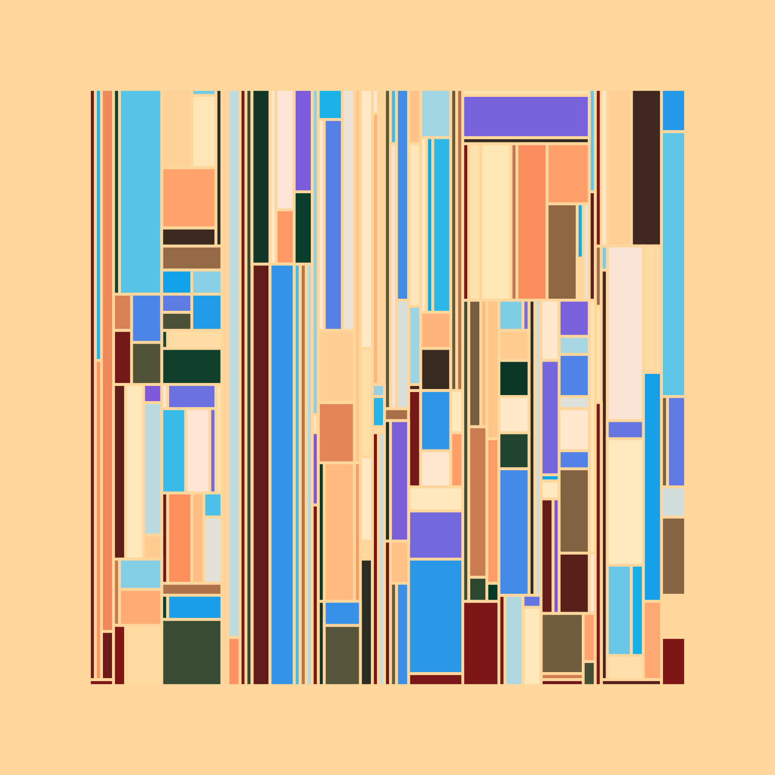
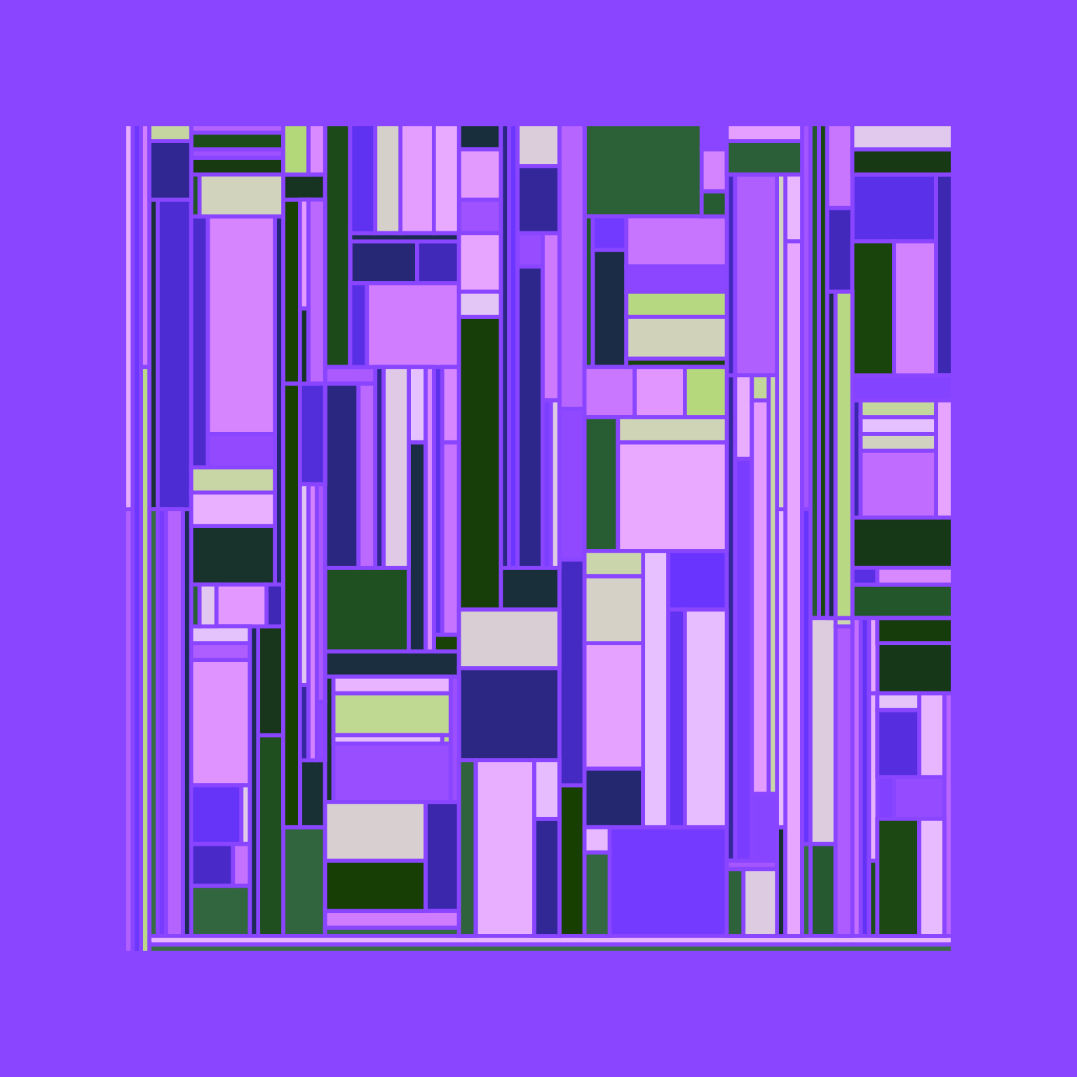
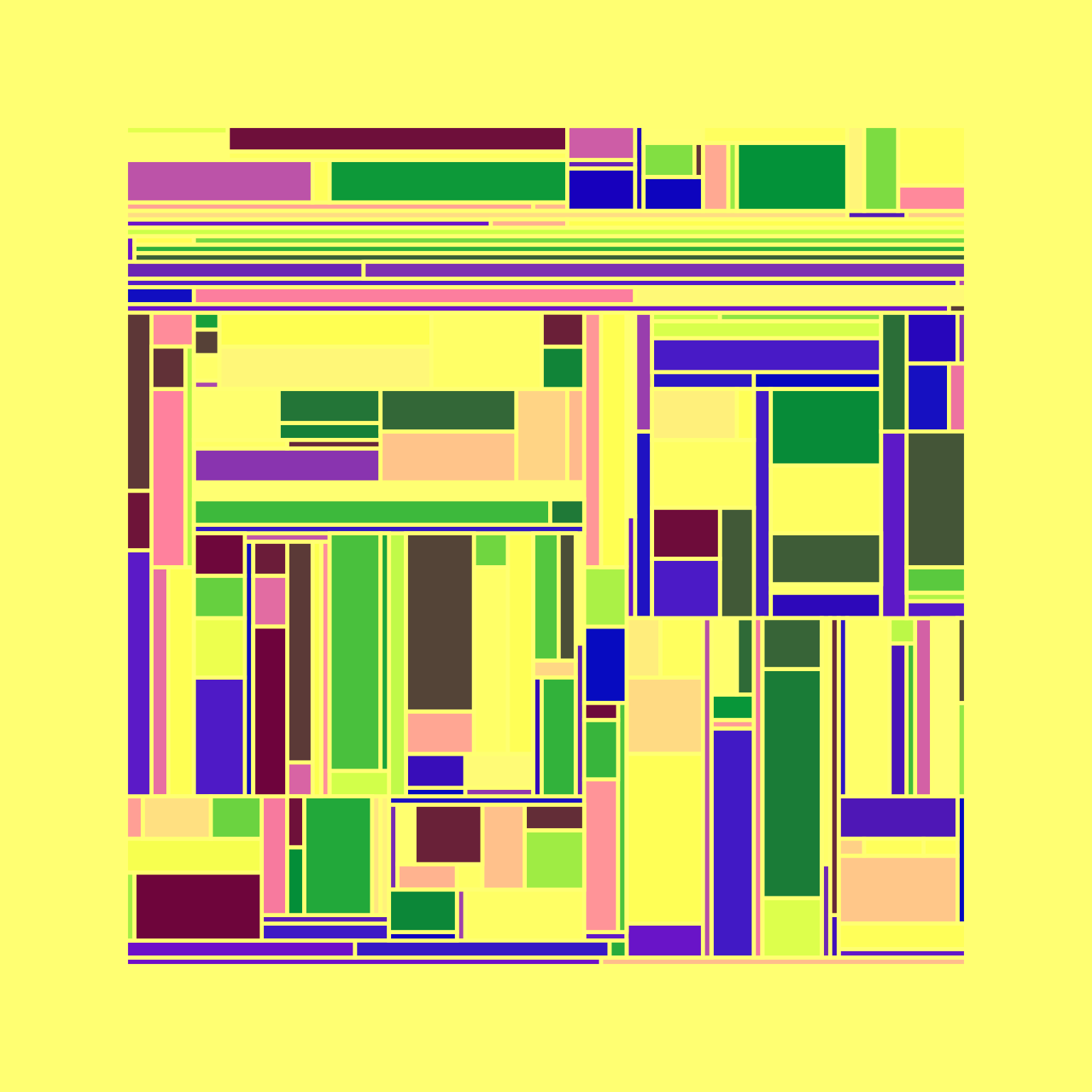
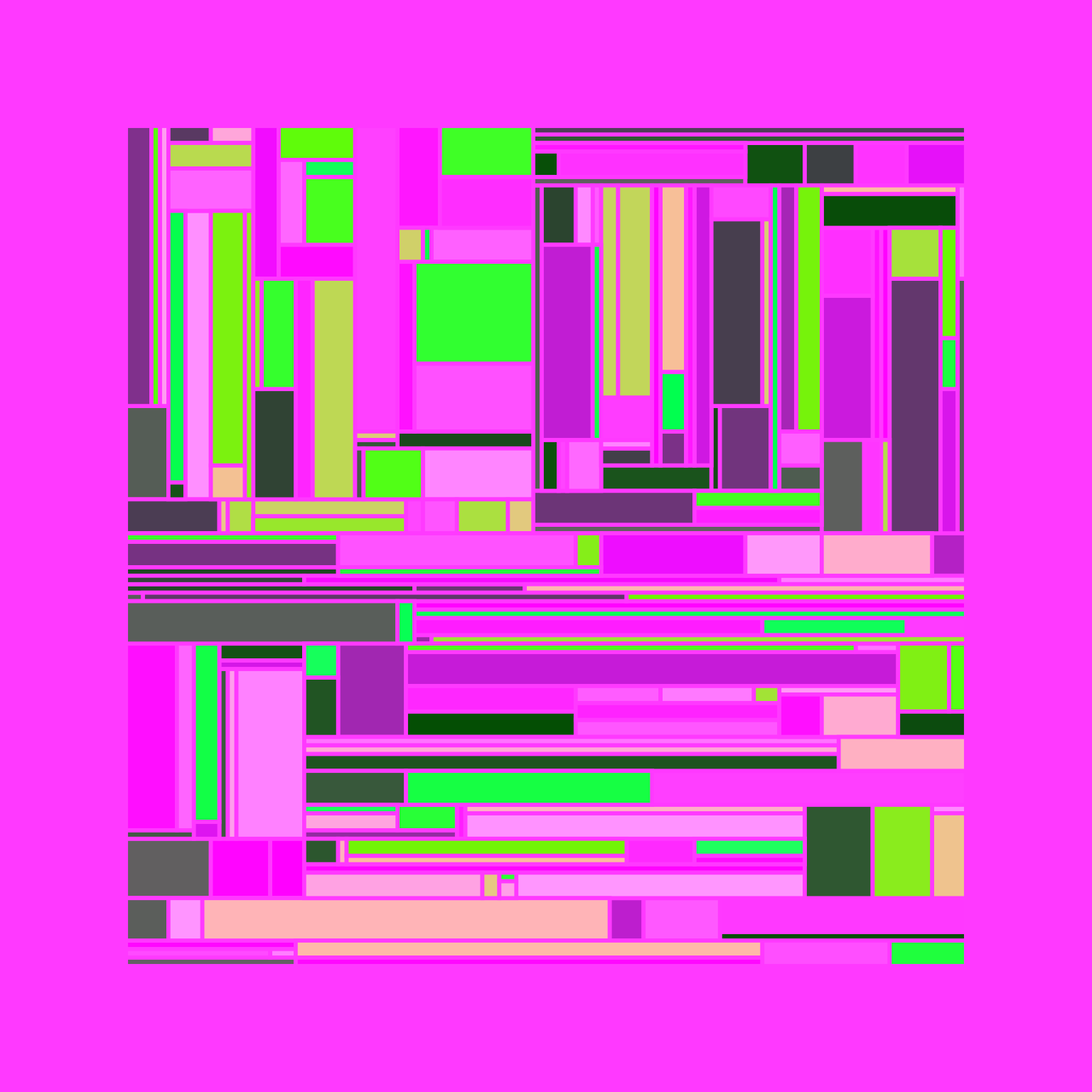
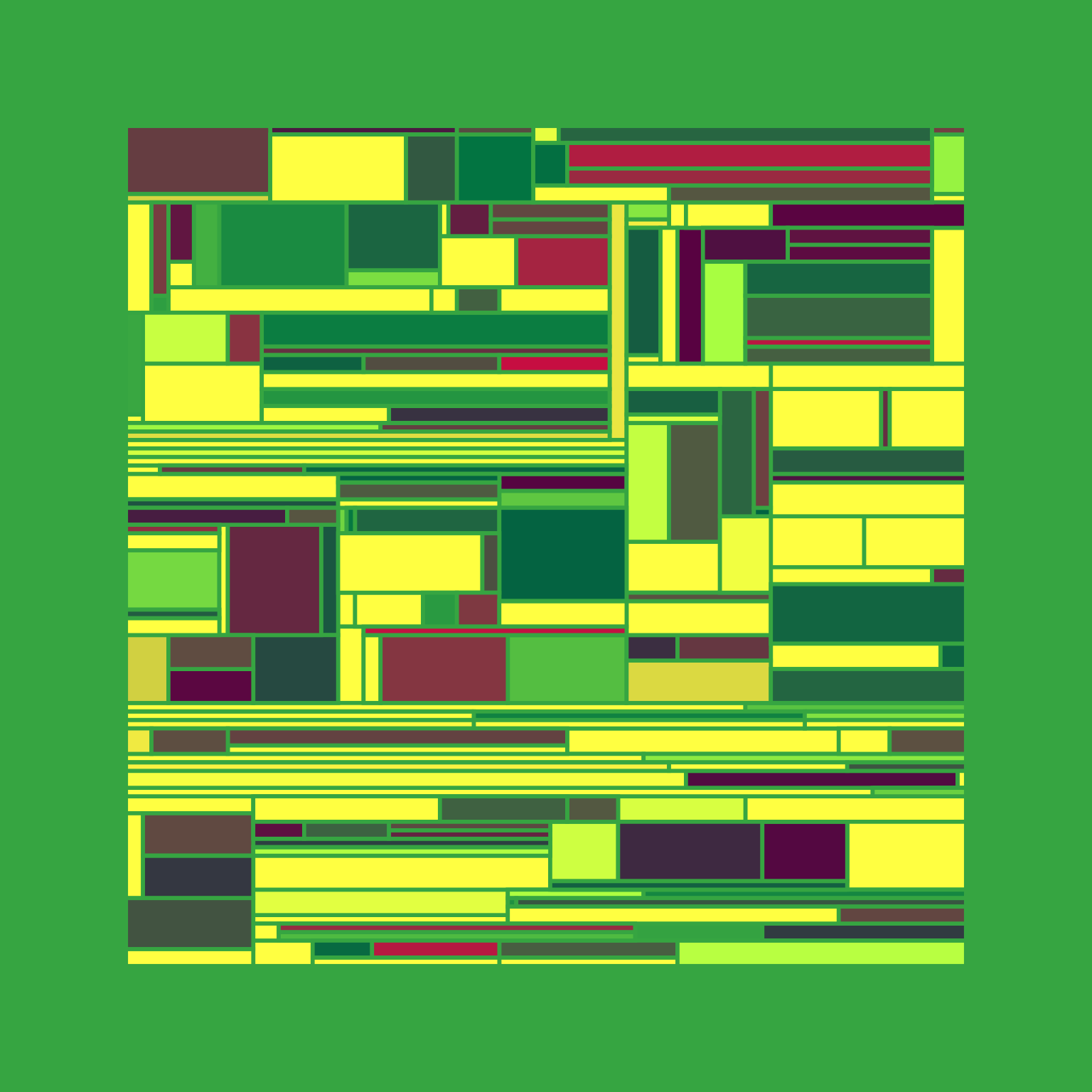
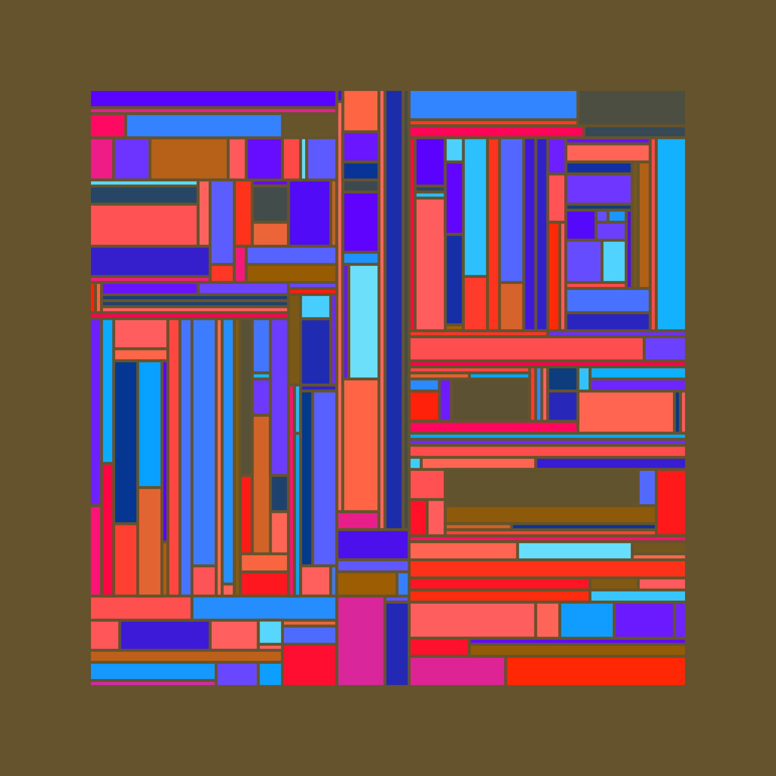
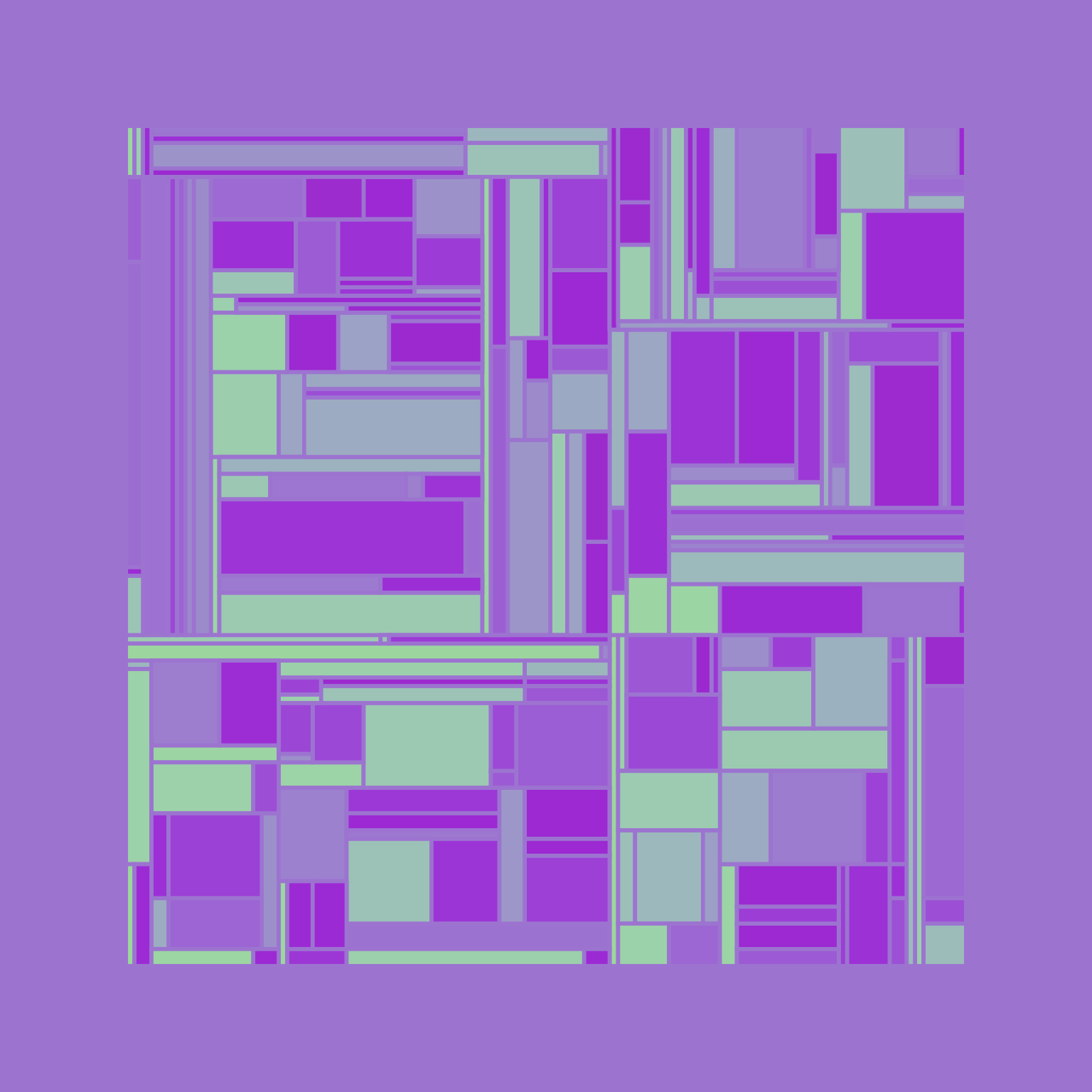
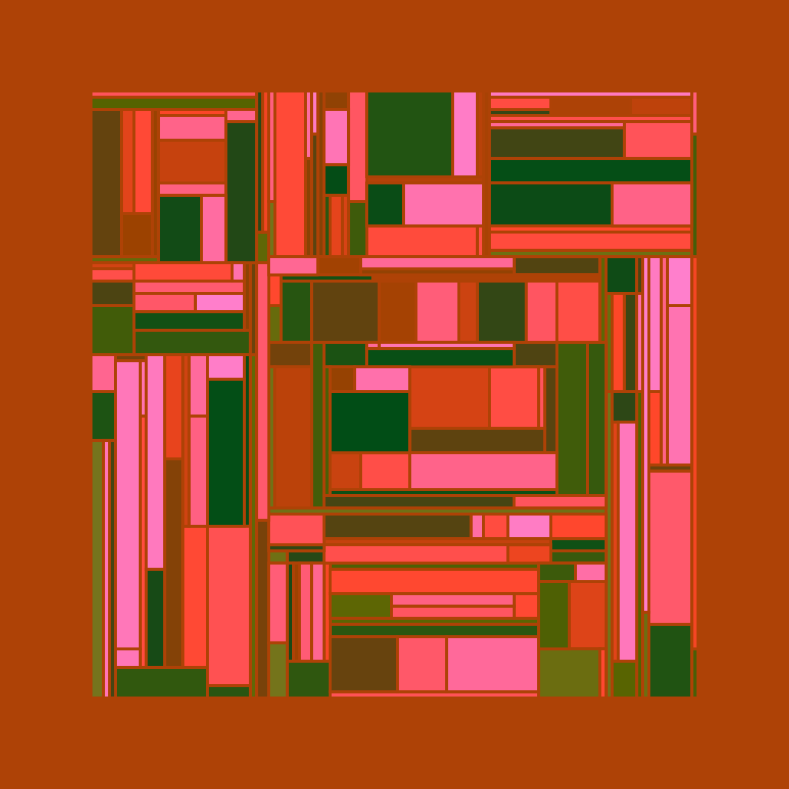
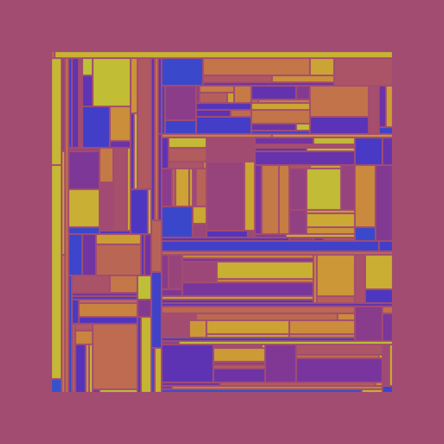
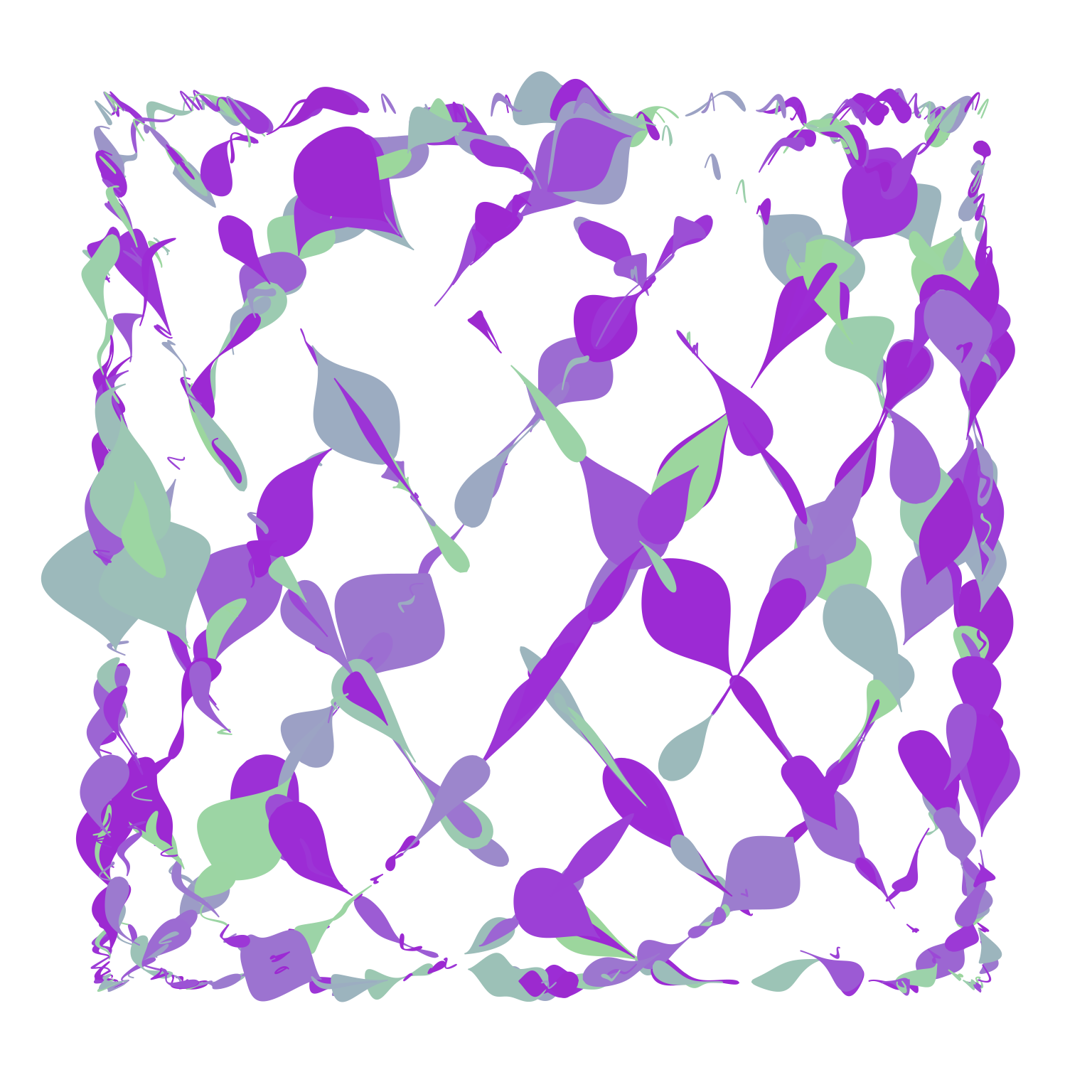
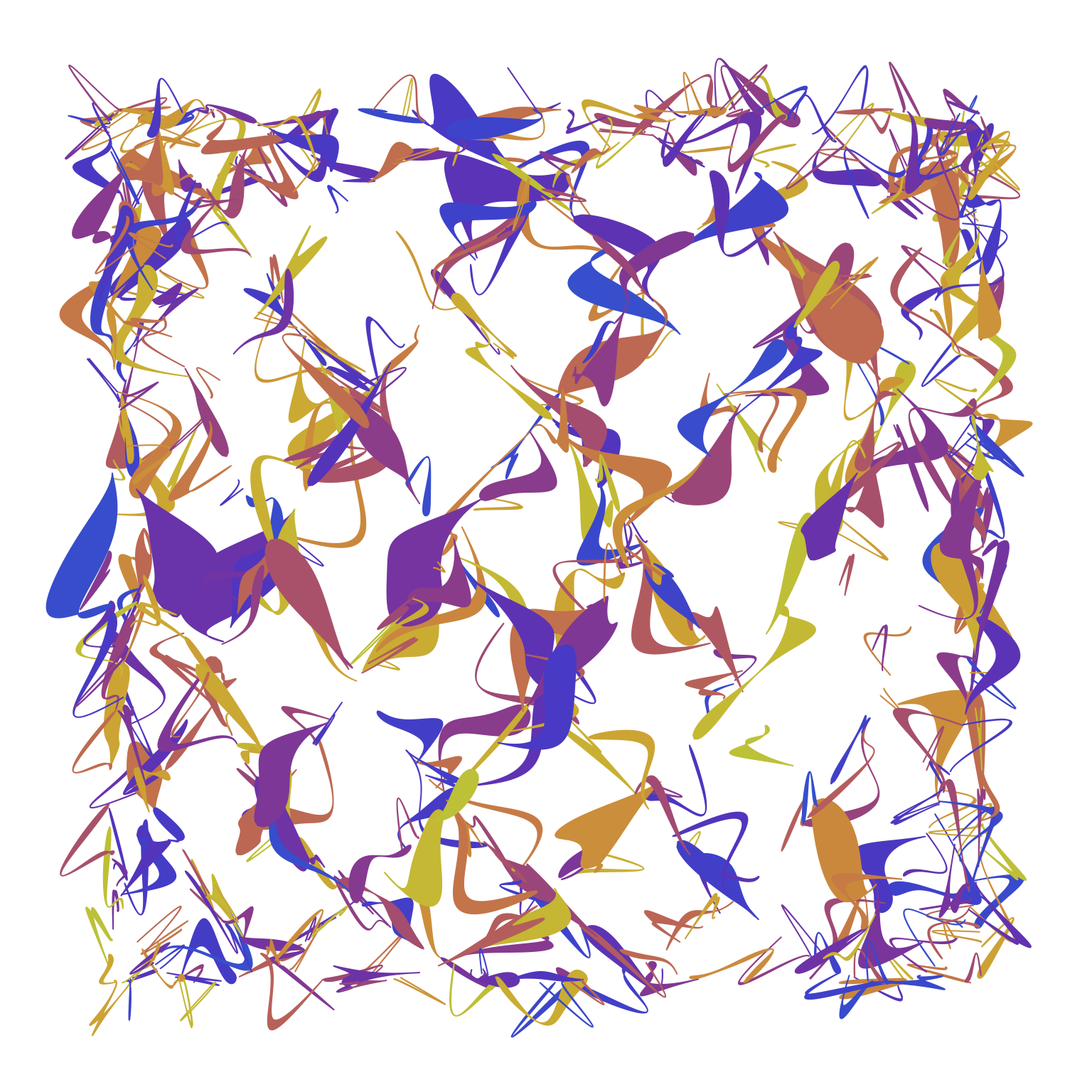
To get a feel for how these palettes behave when used in generative art, here are some pieces created using them. These pieces are created using the subdivision() system that I wrote about as part of the art from code workshop I gave a few years ago.

choose_rectangle <- function(blocks) {
  sample(nrow(blocks), 1, prob = blocks$area)
}

choose_break <- function(lower, upper) {
  round((upper - lower) * runif(1))
}

create_rectangles <- function(left, right, bottom, top, value) {
  tibble::tibble(
    left = left,
    right = right,
    bottom = bottom,
    top = top,
    width = right - left,
    height = top - bottom,
    area = width * height,
    value = value
  )
}

split_rectangle_x <- function(rectangle, new_value) {
  with(rectangle, {
    split <- choose_break(left, right)
    new_left  <- c(left, left + split)
    new_right <- c(left + split, right)
    new_value <- c(value, new_value)
    create_rectangles(new_left, new_right, bottom, top, new_value)
  })
}

split_rectangle_y <- function(rectangle, new_value) {
  with(rectangle, {
    split <- choose_break(bottom, top)
    new_bottom <- c(bottom, bottom + split)
    new_top <- c(bottom + split, top)
    new_value <- c(value, new_value)
    create_rectangles(left, right, new_bottom, new_top, new_value)
  })
}

split_rectangle <- function(rectangle, value) {
  split_fn <- ifelse(runif(1) < .5, split_rectangle_x, split_rectangle_y)
  split_fn(rectangle, value)
}

split_block <- function(blocks, value) {
  old <- choose_rectangle(blocks) 
  new <- split_rectangle(blocks[old, ], value)
  dplyr::bind_rows(blocks[-old, ], new)
}

subdivision <- function(ncol = 100, 
                        nrow = 100, 
                        nsplits = 256,
                        border = NULL, 
                        seed = NULL) {
  
  if (!is.null(seed)) set.seed(seed)

  pal <- cosine_palette(n = 256, seed = seed)

  if (is.null(border)) border <- pal[128]

  rct <- create_rectangles(
    left = 1, 
    right = ncol, 
    bottom = 1, 
    top = nrow, 
    value = 0
  )

  div <- purrr::reduce(
    1:nsplits, 
    split_block, 
    .init = rct
  )

  plt <- div |> 
    ggplot2::ggplot(ggplot2::aes(
      xmin = left, 
      xmax = right, 
      ymin = bottom, 
      ymax = top,
      fill = value
    )) +
    ggplot2::geom_rect(
      show.legend = FALSE, 
      color = border,
      linewidth = 1
    ) +
    ggplot2::scale_fill_gradientn(colours = pal) +
    ggplot2::scale_x_continuous(expand = ggplot2::expansion(mult = .15)) + 
    ggplot2::scale_y_continuous(expand = ggplot2::expansion(mult = .15)) + 
    ggplot2::coord_equal() +
    ggplot2::theme_void() +
    ggplot2::theme(plot.background = ggplot2::element_rect(
      color = border,
      fill = border
    ))

  plt
}

seeds |> purrr::walk(\(s) plot(subdivision(seed = s)))

Not too bad at all. Some of the pieces are pretty awful, a few of them are lovely, and most are okay. Given that I’ve made no attempt at all to optimise the way that palette aligns with the structure of the pieces, that’s not a bad outcome at all.

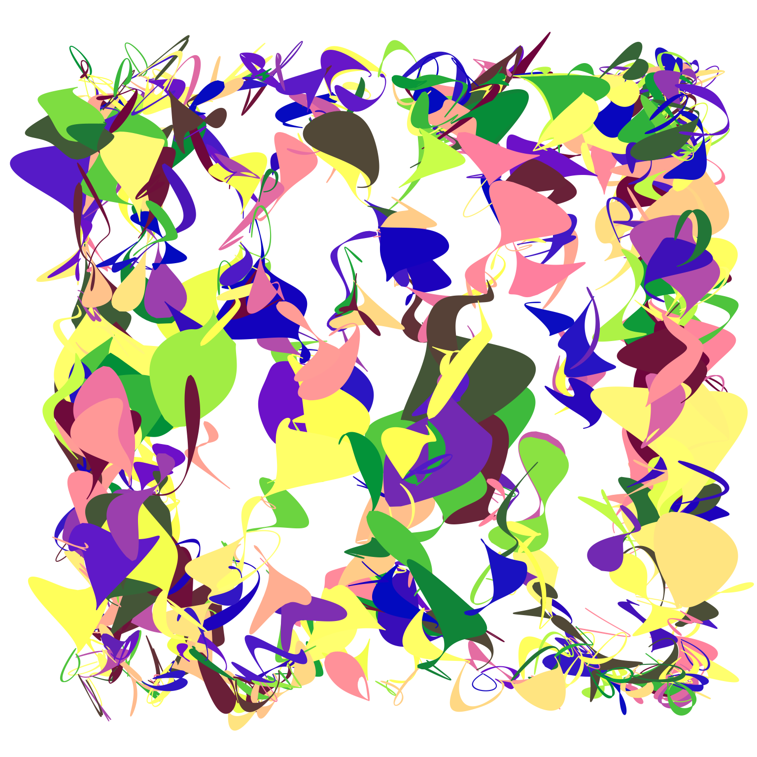
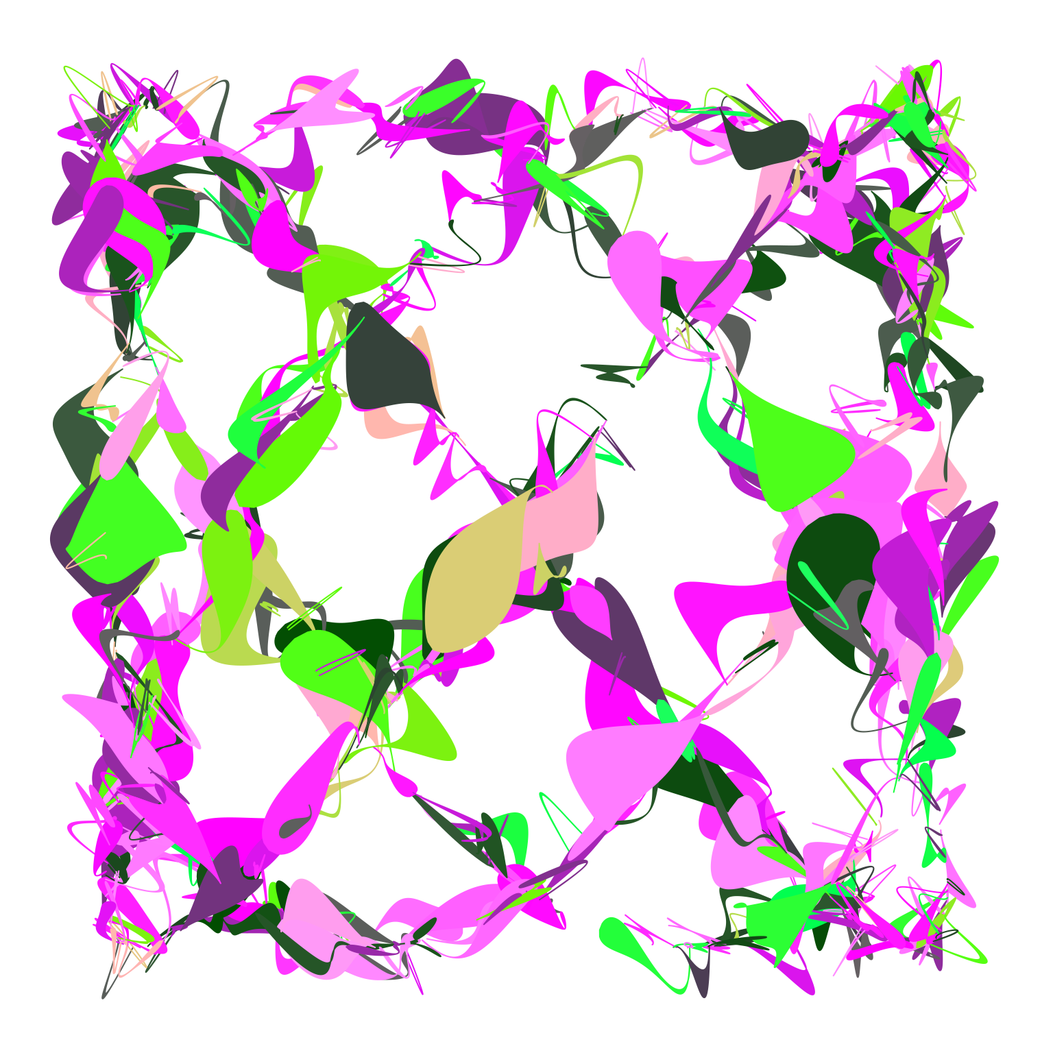
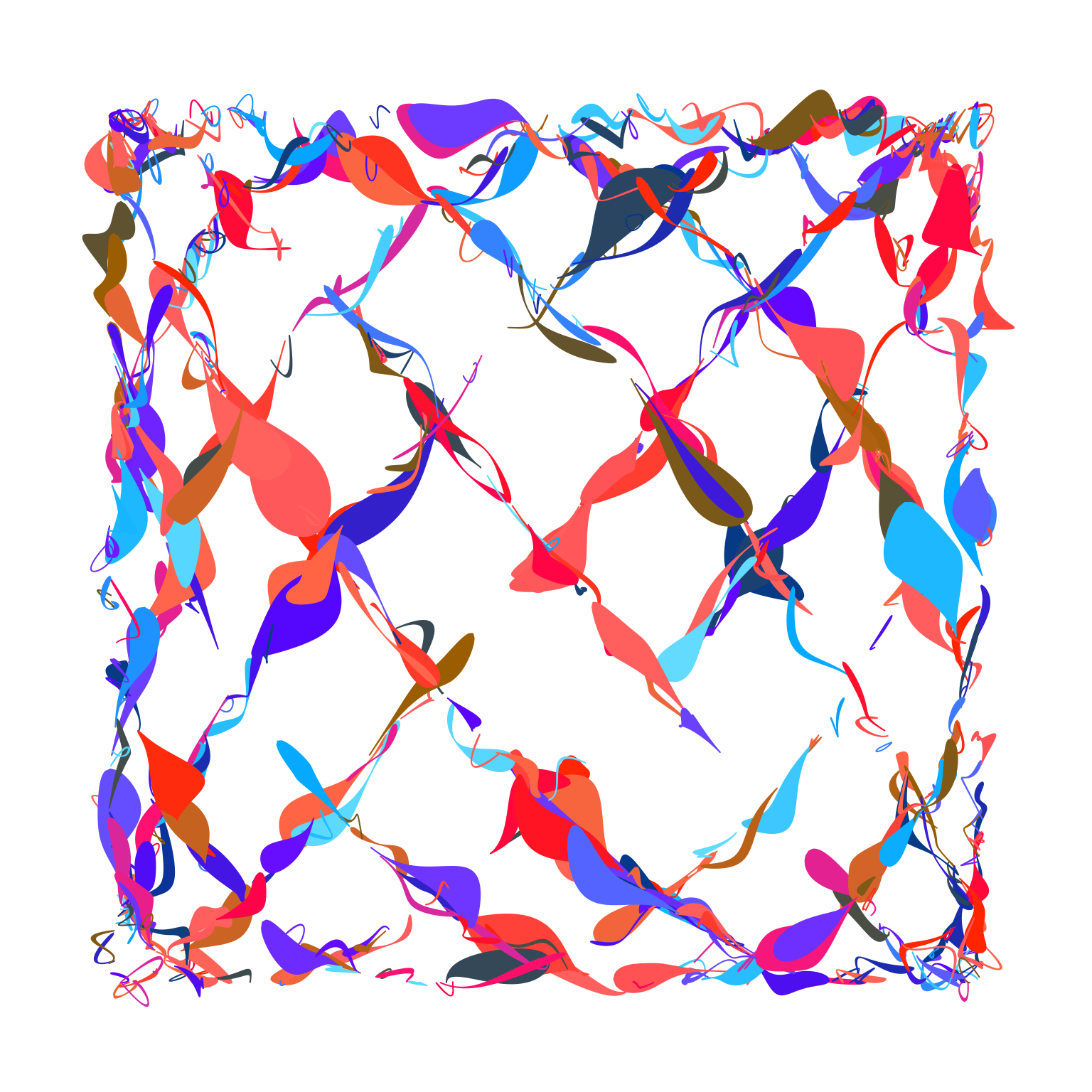
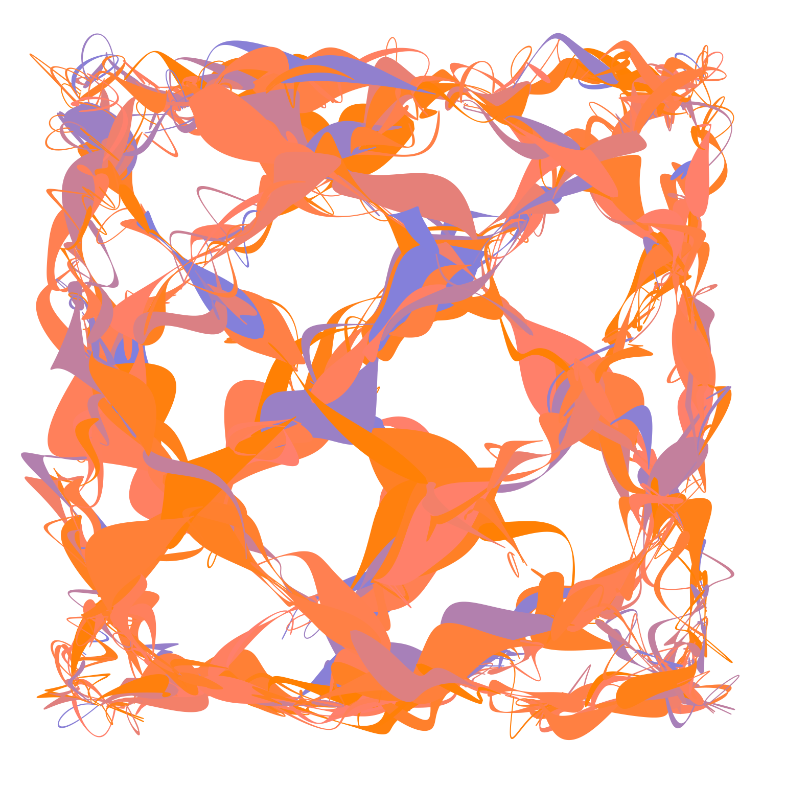
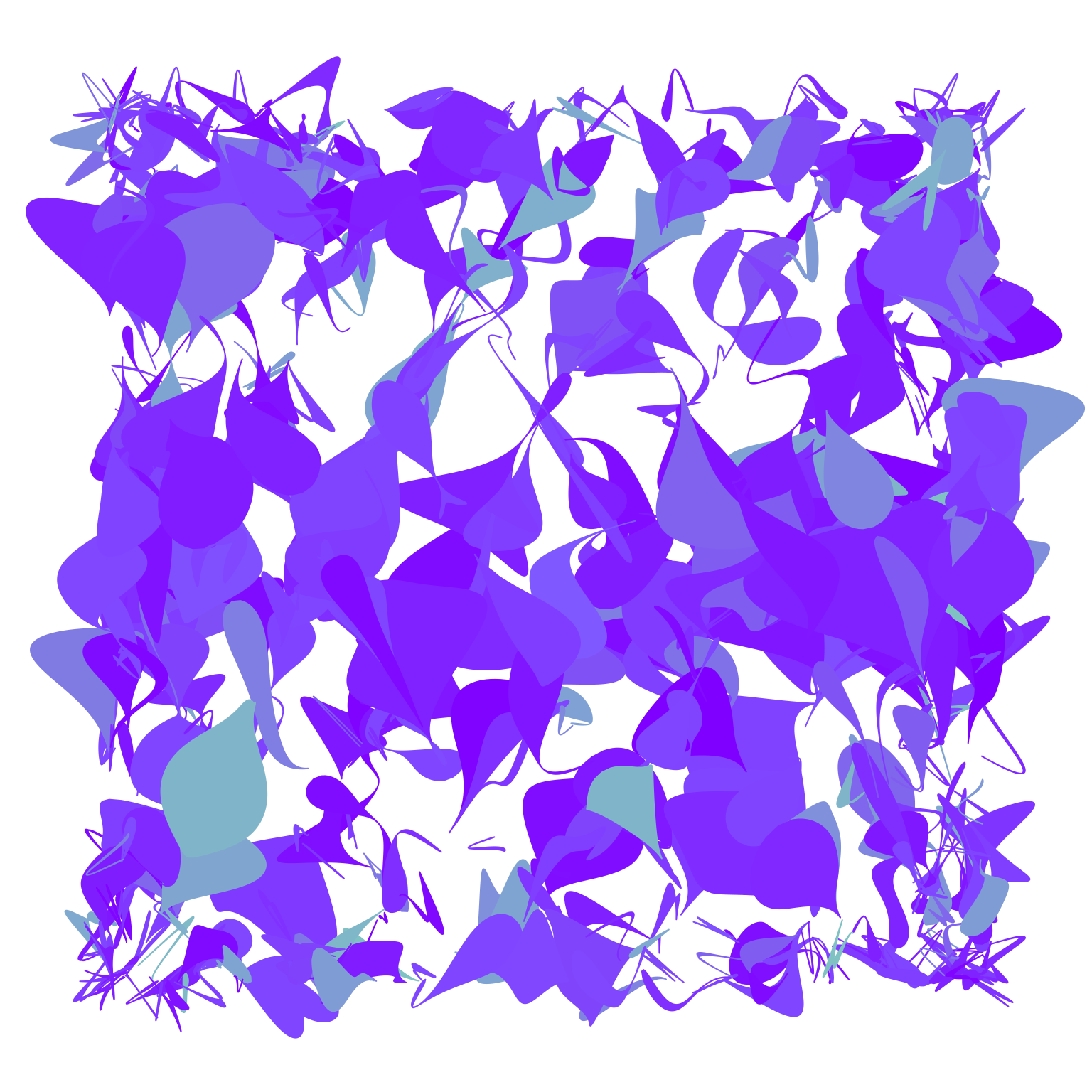
As a second example, here’s a series of pieces based on the lissajous system, all using the same palettes:

seeds |> purrr::walk(\(s) lissajous(seed = s))

Also pretty tolerable. In any specific application I’d probably want to tinker a bit and adapt to the specific aesthetic that the system is targeting, but I’m not displeased at all. For something so simple it works better than I expected. Okay, all good. We’re done now. Post completed, nothing else to add. Somehow I have managed to write a short blog post without turning it into a computational novella, and the whole exercise only took a few hours from beginning to end. 🎉