
library(rxode2)
library(tibble)
library(ggplot2)
library(microbenchmark)Hello, yes, this is another pharmacometrics post. There have been quite a few of these lately as I try to bring myself up to speed on a new discipline. This one is about the rxode2 package, a pharmacometric simulation tool and the successor to the widely-used RxODE package.1 Although the original RxODE package is now archived on CRAN, the syntax for rxode2 is very similar, and as far as I can tell it’s fairly (fully?) backward-compatible with the older package.
Installation
As with other packages for pharmacometric simulation such as mrgsolve, models defined with rxode2 need to be compiled before they are run, and so when you install the package you need the appropriate build tools. There are some implications to this. The package is on CRAN, so you can install it with:
install.packages("rxode2")However, like most R packages that allow you to compile C/C++/Fortran/Rust/Your-Favourite-Language-Here code, it relies heavily on system dependencies that you may or may not have, and managing the build tools is an OS-specific thing. I’m running Ubuntu 22.04, and (for reasons that don’t bear mentioning) I recently did a “factory reset”2 and did a fresh install of Ubuntu. So, yeah, I didn’t have everything I needed. Yes, I did have the gcc compiler installed, but that’s not the only system dependency you have to care about. In my case, I was missing gfortran, libblas, and liblapack. As a consequence, when I tried to run the example code on the package website, all I got was a long stream of error messages. In order to get started, I had to do this:
sudo apt install gfortran libblas-dev liblapack-dev liblapack-docThat worked for me, but I make no promises that it will work for you. Caveat emptor and all that.3 But let’s not stand on installation formalities when there are simulations to run. It is time to load some packages and dive once more into the abyss…
The rxode2 mini-language
I don’t understand
You claiming I’m a handful when you show up all empty-handed
The way you say you love me like you’ve just been reprimanded
’Cause I know you like mind games
– BANKS

The story begins with a little commentary on the slippery nature of R as a programming language. It’s not exactly news to many people at this point, but R is famous4 for the extremely widespread use of metaprogramming as a tool for implementing domain-specific languages within R itself.5 As a consequence of this, the same code can have different meaning when called in different contexts. It’s both a curse and a blessing: one the one hand it makes R very flexible in a way that is convenient for analysts, but on the other hand it can be a bit confusing to people from a more conventional programming background who don’t expect R to work this way.
The use of domain-specific languages in pharmacometric modelling is not uncommon: for instance, in my previous post about mrgsolve, I talked about the mini-language used to specify models in that package. Not surprisingly, rxode2 has its own mini-language with it’s own custom syntax. In mrgsolve, you can specify a model by writing the code for it in a separate file, or passing it as a string within R. You can do that with rxode2 too, but rxode2 also allows you to pass the model specification as a code block: a collection of statements enclosed in curly braces and treated as a single expression. Here’s an example of how that works:
mod <- rxode2({
  # initial values for all four "compartments"
  depot(0) = 0;
  central(0) = 0;
  peripheral(0) = 0;
  auc(0) = 0;

  # drug concentrations
  CP = central / VC;    # central compartment concentration
  PP = peripheral / VP; # peripheral compartment concentration

  # differential equations
  d/dt(depot)       = -(KA * depot);
  d/dt(central)     =  (KA * depot) - (Q * CP) + (Q * PP) - (CL * CP);
  d/dt(peripheral)  =  (Q * CP) - (Q * PP);
  d/dt(auc)         =  CP;
})
If you don’t look at it too closely you might think this is regular R code, but… it isn’t. The code contained within the braces is captured by the rxode2() function, and then interpreted according to the rules of the mini-language. We’ll need to take a moment to unpack the mini-language itself, but that can wait.
Let’s start by looking at this as a pharmacometrician might. Notice that although this is a two-compartment model in pharmacometric terms, from the perspective of rxode2 there are four “compartments” that define the state of the system. In addition to the usual two compartments (central and peripheral), there is an extravascular depot compartment used to model drug intake. For instance, for an orally-administered drug the depot compartment would be the gut.6 The depot compartment is “real” in the sense that it is loosely intended to correspond to something in the physical system that we’re modelling. By convention we don’t consider it to be one of the pharmacokinetic compartments, but it’s still a real thing. In contrast, the auc “compartment” has no physical analog at all. It’s included so that the model keeps track of the accumulated drug exposure.7 As I’m quickly coming to learn, this is a very handy trick when running pharmacometric simulations.
Now that we’ve looked at it as an analyst, let’s look at it as a programmer. The syntax within the rxode2 model specification is not “real” R code. The statements enclosed within the curly braces look vaguely R-like, but if you tried to evaluate these expressions outside the context of the rxode2() function, you’d get errors. Thanks to the magic of non-standard evaluation in R, the rxode2() function is able capture the code before it is evaluated, and prevents R from evaluating it the way it normally would. Instead of following the regular rules of R, it follows the syntax provided by the rxode2 mini-language. This mini-language is similar to R in some ways:
- Assignment statements can use
=or<-as the assignment operator.8 - Comments are specified using the hash (
#) character - Semi-colon characters (
;) are optional, and specify the end of a line
However, there are specialised statements used in the mini-language that don’t exist in regular R code. For example, there are two kinds of special statements I’ve used in this code:
- Time-derivative statements (i.e., the ones that have something like
d/dt(central)on the left hand side) are used to specify the differential equations in the ODE system. - Initial-condition statements (i.e., the ones where I set something like
central(0)on the left hand side) are used to specify the initial state of the ODE system.
You can check the rxode2 syntax page for more information about the mini-language and what other kinds of special statements exist.
The rxode2 model object
In the previous section I used the rxode2() function to specify a pretty standard two-compartment pharmacokinetic model, and assigned the resulting model object to a boringly-named variable called mod.9 The model object is the primary vehicle for interfacing with the compiled code from R, so it’s helpful to take a look at it:
modrxode2 2.0.13 model named rx_7b738a16dd646d432336a380787bd163 model (✔ ready).
x$state: depot, central, peripheral, auc
x$params: VC, VP, KA, Q, CL
x$lhs: CP, PP
Again, there are a few things to unpack in this output:
- The first line of the output has some technical information about the model. It tells us what version of rxode2 was used to build the model, gives us the name of the built model (see below), and tells us that it’s ready to use.10
- The second line tells us about
mod$state, which in this case are the four “compartment” variables that comprise the state vector for the underlying ODE system. - The third line tells us about
mod$params, the list of parameters that need to be passed to the model as input to the simulation - The fourth line tells us about
mod$lhs, the list of additional defined variables that are created by the model and whose value will be recorded in the output.
Like many R packages that generate compiled code, rxode2 manages the compiled object for you. The long unintelligible “name” assigned to our model gives us the hint we need to find the compiled objects. Within the R session temp directory, the rxode2 package has created an “rxode2” subfolder.11 And indeed, if I take a peek at the contents of this folder, I find something with an identical name:
fs::dir_ls(fs::path(tempdir(), "rxode2"))/tmp/RtmpC0i8oK/rxode2/018374b1ca9115fbc3be9f765f32e47f.md5
/tmp/RtmpC0i8oK/rxode2/rx_7b738a16dd646d432336a380787bd163__.rxd
Okay, makes sense.
Event tables
Event tables (also called event schedules) are the primary way the user specifies things that happen in the simulation. These mostly consist of two kinds of event: dosing events, where the drug is administered, and observation events, where the state of the system is measured. In the rxode2 package these are specified with the et() function, and you can use the pipe operator to build up complex event schedules. I’ll take my example from the rxode2 documentation, and walk through it slowly. One nice thing about the event schedules in rxode2 is that you can specify units, so we’ll start with an event table that doesn’t contain any actual events, but specifies the units in which those events will be expressed:
events <- et(amountUnits = "mg", timeUnits = "hours")
events
── EventTable with 0 records ──
0 dosing records (see x$get.dosing(); add with add.dosing or et)
0 observation times (see x$get.sampling(); add with add.sampling or et)
The output here isn’t super exciting, since there are no actual events encoded here. But it does let me mention one nice little feature of rxode2: the print methods are generally quite informative, and have nice little “nudges” like the ones you can see above that can help new (or even experienced) users work out what they might need to do next.
Anyway, let’s add some dosing events, shall we? Let’s assume an initial dose of amt = 10000 (in milligrams) is administered at time = 0, and repeated for an additional 9 times at 12 hour intervals (i.e., addl = 9, ii = 12). In the interests of being explicit, I’ll set cmt = "depot" to be clear about which compartment the dose is administered to.
events <- events |>
  et(time = 0, amt = 10000, addl = 9, ii = 12, cmt = "depot")

events
── EventTable with 1 records ──
1 dosing records (see x$get.dosing(); add with add.dosing or et)
0 observation times (see x$get.sampling(); add with add.sampling or et)
multiple doses in `addl` columns, expand with x$expand(); or etExpand(x)
── First part of x: ──
# A tibble: 1 × 6
time cmt amt ii addl evid
<dbl> <chr> <dbl> <dbl> <int> <evid>
1 0 depot 10000 12 9 1:Dose (Add)
This format for an event table – where time, amt, addl, and ii are used to specify a sequence of regularly spaced dosing events in a single row – will seem quite familiar to anyone in the field, and since I’ve talked about this notation in previous posts, I’ll not bore people by explaining it yet again.
Moving along, let’s also assume that after 120 hours has passed (time = 120) the dosing schedule changes: the dose drops to amt = 2000 milligrams, the interdose interval is increased slightly to ii = 14 hours, and this dosing regime is maintained for addl = 4 additional doses (i.e., 5 in total). So now we have this:
events <- events |>
  et(time = 120, amt = 2000, addl = 4, ii = 14, cmt = "depot")

events
── EventTable with 2 records ──
2 dosing records (see x$get.dosing(); add with add.dosing or et)
0 observation times (see x$get.sampling(); add with add.sampling or et)
multiple doses in `addl` columns, expand with x$expand(); or etExpand(x)
── First part of x: ──
# A tibble: 2 × 6
time cmt amt ii addl evid
<dbl> <chr> <dbl> <dbl> <int> <evid>
1 0 depot 10000 12 9 1:Dose (Add)
2 120 depot 2000 14 4 1:Dose (Add)
Now that we have specified all the dosing events, we need to add the “observation” events. In a real study, observation times would be the times at which we take a real-world measurement of some kind, but in the context of the simulation it’s just a set of times at which the state of the system is computed. Let’s compute the state of the system for the first 300 hours:
events <- events |> et(time = 0:300)
events
── EventTable with 303 records ──
2 dosing records (see x$get.dosing(); add with add.dosing or et)
301 observation times (see x$get.sampling(); add with add.sampling or et)
multiple doses in `addl` columns, expand with x$expand(); or etExpand(x)
── First part of x: ──
# A tibble: 303 × 6
time cmt amt ii addl evid
<dbl> <chr> <dbl> <dbl> <int> <evid>
1 0 (obs) NA NA NA 0:Observation
2 0 depot 10000 12 9 1:Dose (Add)
3 1 (obs) NA NA NA 0:Observation
4 2 (obs) NA NA NA 0:Observation
5 3 (obs) NA NA NA 0:Observation
6 4 (obs) NA NA NA 0:Observation
7 5 (obs) NA NA NA 0:Observation
8 6 (obs) NA NA NA 0:Observation
9 7 (obs) NA NA NA 0:Observation
10 8 (obs) NA NA NA 0:Observation
# ℹ 293 more rows
And now we’re done. We have a complete events table that can be used in our simulation. Admittedly, I went through that awfully slowly. The whole thing could have been bundled into a single pipeline like this:
events <- et(amountUnits = "mg", timeUnits = "hours") |>
  et(time = 0, amt = 10000, addl = 9, ii = 12, cmt = "depot") |>
  et(time = 120, amt = 2000, addl = 4, ii = 14, cmt = "depot") |>
  et(time = 0:300)
Simulating one subject
I was alone, falling free
Trying my best not to forget
What happened to us
What happened to me
– Placebo12
We’re now almost at a point where we can run a simple simulation using the model specified via the mod object, and the events table in events. The only thing we haven’t done yet is specify pharmacokinetic parameters that need to be passed to the model as input. To keep things simple, I’ll simulate only a single subject, and so the input parameters will be passed as a table with one row corresponding to our lone subject, and one column per parameter that needs to be specified. If we look at the model spec we can see that requires all of the following to be given:
- elimination clearance (
CL) - absorption rate constant (
KA) - intercompartmental clearance (
Q) - volume of distribution for the central compartment (
VC) - volume of distribution for the peripheral compartment (
VP)
Indeed, if we take a look at mod$params we see the same listing:
mod$params[1] "VC" "VP" "KA" "Q" "CL"Okay, so let’s put together a one-row data frame params containing all these parameters for a single simulated subject:
params <- tibble(
  KA = 0.294,
  CL = 18.6,
  VC = 40.2,
  VP = 297,
  Q = 10.5
)
params
# A tibble: 1 × 5
KA CL VC VP Q
<dbl> <dbl> <dbl> <dbl> <dbl>
1 0.294 18.6 40.2 297 10.5
Now that we have our parameters, we’re ready to go. There are several ways you can call the solver and run the simulation (documentation here), but I’m currently quite partial to calling solve(),13 like so:
out <- solve(mod, params, events)When we print out, we get a fairly detailed description of the simulation that includes information about the parameters and the initial state:
out── Solved rxode2 object ──
── Parameters (x$params): ──
VC VP KA Q CL
40.200 297.000 0.294 10.500 18.600
── Initial Conditions (x$inits): ──
depot central peripheral auc
0 0 0 0
── First part of data (object): ──
# A tibble: 301 × 7
time CP PP depot central peripheral auc
<dbl> <dbl> <dbl> <dbl> <dbl> <dbl> <dbl>
1 0 0 0 10000 0 0 0
2 1 44.4 0.920 7453. 1784. 273. 26.4
3 2 54.9 2.67 5554. 2206. 794. 77.7
4 3 51.9 4.46 4140. 2087. 1324. 132.
5 4 44.5 5.98 3085. 1789. 1776. 180.
6 5 36.5 7.18 2299. 1467. 2132. 221.
# ℹ 295 more rows
Extremely pretty print method notwithstanding, under the hood it’s nothing fancy. It’s a regular data frame with a few extra classes and some metadata, which means we can pass it straight to ggplot without any coercion, and draw a pretty picture:
ggplot(out, aes(time, CP)) +
  geom_area(linewidth = 1) +
  ylab("concentration") +
  theme_bw()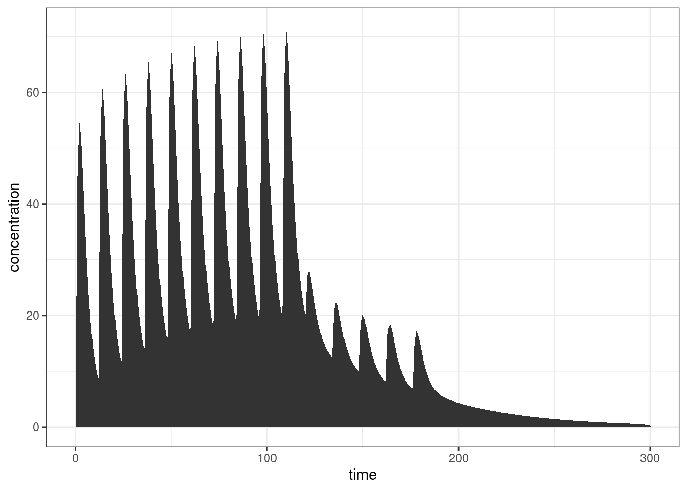
Yep, that looks about right.

Simulating multiple subjects
I like big boys, itty bitty boys
Mississippi boys, inner city boys
I like the pretty boys with the bow tie
Get your nails did, let it blow dry
I like a big beard, I like a clean face
I don’t discriminate, come and get a taste
From the playboys to the gay boys
Go and slay, boys, you my fave boys
–Lizzo
The previous example shows how to simulate a single subject. However, the world is full of lots of different people with different characteristics, so in a more realistic simulation scenario we would want to simulate many people with different parameter values. In order to accommodate this, the parameter table now has multiple rows:
params <- tibble(
  KA = rnorm(20, mean = 0.294, sd = 0.03),
  CL = rnorm(20, mean = 18.6, sd = 2),
  VC = rnorm(20, mean = 40.2, sd = 2),
  VP = rnorm(20, mean = 297, sd = 10),
  Q = rnorm(20, mean = 10.5, sd = 1)
)
params
# A tibble: 20 × 5
KA CL VC VP Q
<dbl> <dbl> <dbl> <dbl> <dbl>
1 0.275 20.4 39.9 321. 9.93
2 0.300 20.2 39.7 297. 10.4
3 0.269 18.7 41.6 304. 11.7
4 0.342 14.6 41.3 297. 8.98
5 0.304 19.8 38.8 290. 11.1
6 0.269 18.5 38.8 299. 10.8
7 0.309 18.3 40.9 279. 11.6
8 0.316 15.7 41.7 312. 10.2
9 0.311 17.6 40.0 299. 10.9
10 0.285 19.4 42.0 319. 10.8
11 0.339 21.3 41.0 302. 9.96
12 0.306 18.4 39.0 290. 11.7
13 0.275 19.4 40.9 303. 11.7
14 0.228 18.5 37.9 288. 11.2
15 0.328 15.8 43.1 284. 12.1
16 0.293 17.8 44.2 300. 11.1
17 0.294 17.8 39.5 293. 9.22
18 0.322 18.5 38.1 297. 9.93
19 0.319 20.8 41.3 298. 9.28
20 0.312 20.1 39.9 291. 10.0
The command to run the simulation remains unchanged:
out <- solve(mod, params, events)I’ll show you the out object in a moment, but it’s probably easier to understand it if we start with a plot:
out |>
  dplyr::mutate(sim.id = paste("Subject", sim.id)) |>
  ggplot(aes(time, CP, fill = sim.id)) +
  geom_area(linewidth = 1, show.legend = FALSE) +
  facet_wrap(~ sim.id, nrow = 5) +
  labs(x = "Time", y = "Concentration") +
  theme_bw()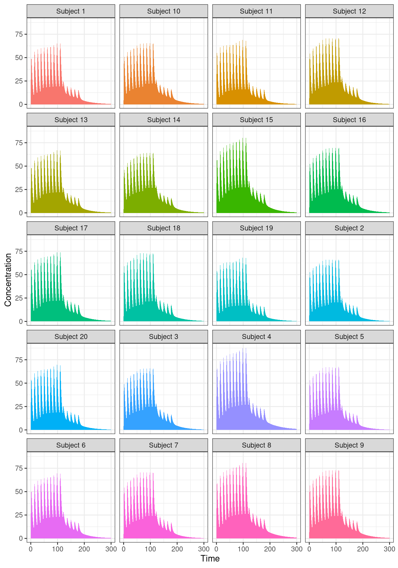
As you can see, all 20 subjects have qualitatively similar profiles, but there are noticeable differences in the details. Not surprisingly really. I didn’t build in very much variability into the simulation, and I didn’t even try to incorporate an appropriate covariance structure among the parameters (that’s a topic for another post).14 The main thing that matters here is that we can see that the variation exists.
Anyway, let’s have a look at the table of results out produced by our simulation. As you probably guessed from the ggplot2 code, there’s a column called sim.id that stores the subject identifier, and there are 20 times as many rows as last time, but it’s essentially the same:
out── Solved rxode2 object ──
── Parameters (x$params): ──
# A tibble: 20 × 6
sim.id VC VP KA Q CL
<int> <dbl> <dbl> <dbl> <dbl> <dbl>
1 1 39.9 321. 0.275 9.93 20.4
2 2 39.7 297. 0.300 10.4 20.2
3 3 41.6 304. 0.269 11.7 18.7
4 4 41.3 297. 0.342 8.98 14.6
5 5 38.8 290. 0.304 11.1 19.8
6 6 38.8 299. 0.269 10.8 18.5
7 7 40.9 279. 0.309 11.6 18.3
8 8 41.7 312. 0.316 10.2 15.7
9 9 40.0 299. 0.311 10.9 17.6
10 10 42.0 319. 0.285 10.8 19.4
11 11 41.0 302. 0.339 9.96 21.3
12 12 39.0 290. 0.306 11.7 18.4
13 13 40.9 303. 0.275 11.7 19.4
14 14 37.9 288. 0.228 11.2 18.5
15 15 43.1 284. 0.328 12.1 15.8
16 16 44.2 300. 0.293 11.1 17.8
17 17 39.5 293. 0.294 9.22 17.8
18 18 38.1 297. 0.322 9.93 18.5
19 19 41.3 298. 0.319 9.28 20.8
20 20 39.9 291. 0.312 10.0 20.1
── Initial Conditions (x$inits): ──
depot central peripheral auc
0 0 0 0
Simulation without uncertainty in parameters, omega, or sigma matricies
── First part of data (object): ──
# A tibble: 6,020 × 8
sim.id time CP PP depot central peripheral auc
<int> <dbl> <dbl> <dbl> <dbl> <dbl> <dbl> <dbl>
1 1 0 0 0 10000 0 0 0
2 1 1 41.6 0.757 7594. 1657. 243. 24.7
3 1 2 51.2 2.20 5767. 2041. 705. 72.7
4 1 3 48.4 3.66 4380. 1928. 1176. 123.
5 1 4 41.5 4.93 3326. 1656. 1581. 168.
6 1 5 34.2 5.93 2526. 1362. 1902. 206.
# ℹ 6,014 more rows
As we’ve seen throughout the post, the print method has lots of nice touches. It shows the simulation parameters as well as the simulation results, and has a very gentle message reminding me I haven’t incorporated measurement error, random effects, or parameter uncertainty. Which… I mean, I intentionally left those things out, but actually I do appreciate the clear statement of what wasn’t done here.

Performance considerations
Ain’t no use in trying to slow me down
’Cause you’re running with the fastest girl in town
Ain’t you baby?
– Miranda Lambert
For small simulations like the ones I’m running in this post, you really don’t need to care much about performance. However, when you start running larger simulations it starts to matter a lot. To that end there’s a nice article on speeding up rxode2 in the package documentation which I’ve already found extremely useful at work when doing a little bit of code profiling on analysis code. Since this does matter a fair bit in practice, I’ll walk through the same ideas here.
Let’s define a few functions that run the simulations in different ways. First, I’ll start with a solve_loop() function that deliberately strips out any form of multi-threading. Each row in params is passed as a separate call to solve(), nested inside a for loop:
solve_loop <- function() {
  for(i in 1:nrow(params)) solve(mod, params[i, ], events)
}
This is our baseline case. It’s designed to make life as difficult as possible for rxode2 by enforcing single threaded execution within R. We can improve on this considerably by passing the entire params data frame, allowing rxode2 to run the simulations in parallel. I haven’t looked under the hood to work out exactly how rxode2 manages the parallelism15 Here are three functions that explicitly request 1, 2 or 4 cores/threads:
solve_thread_1 <- function() solve(mod, params, events, cores = 1)
solve_thread_2 <- function() solve(mod, params, events, cores = 2)
solve_thread_4 <- function() solve(mod, params, events, cores = 4)
From experience, I’ve learned that there’s almost never anything to be gained by trying to execute more than four resource-hogging threads simultaneously on my laptop, so I’ll be sensible and won’t try anything more than that. Let’s take a look at the difference in performance for each of these functions:
bench <- microbenchmark(
  solve_loop(),
  solve_thread_1(),
  solve_thread_2(),
  solve_thread_4()
)
bench
Unit: milliseconds
expr min lq mean median uq max neval
solve_loop() 58.630598 62.227245 68.912034 64.780701 68.78793 168.11848 100
solve_thread_1() 8.515051 8.867159 9.635308 9.126248 9.45503 26.11143 100
solve_thread_2() 7.497051 7.720607 8.476758 7.968412 8.44852 15.94618 100
solve_thread_4() 6.538996 7.063265 7.761950 7.160678 7.54286 17.27997 100You can see from looking at the table that there’s a big drop in performance when we force rxode2 to simulate each subject one at a time within a loop: solve_loop() is much, much slower than any of the others. Increasing the number of threads from one to four helps a fair bit too, but not to the same dramatic extent. This is even more apparent when we visualise the results:
autoplot(bench)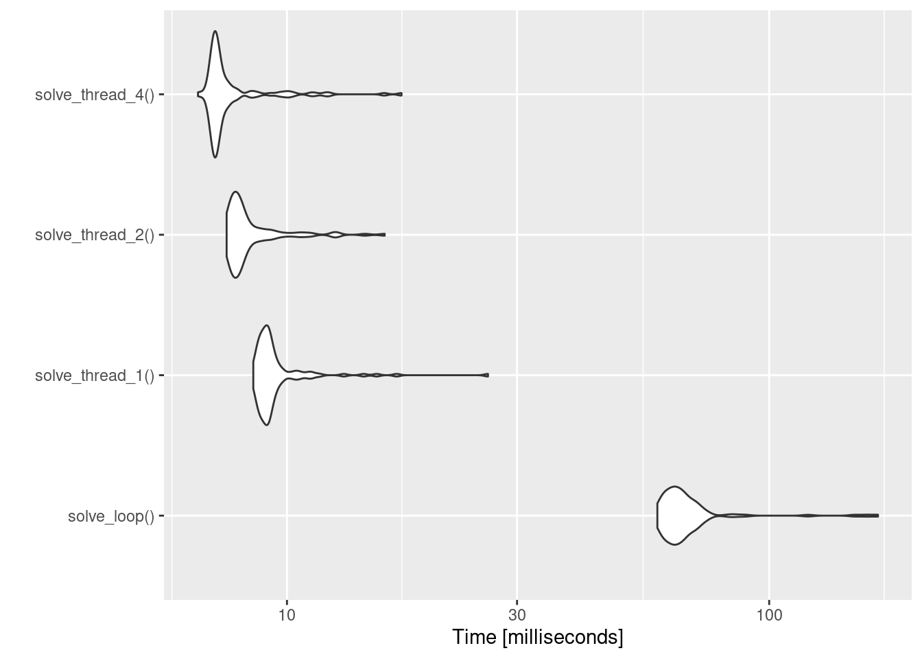
Admittedly, the time scale here is such that it doesn’t really matter much, but for more realistic examples I’ve played with the speed-up seems to be pretty similar and it can make a big difference to the performance of analysis code.
Footnotes
As an aside: when getting started, I found it a little easier to look at the rxode2 user manual than to work from the pkgdown site. As far as I can tell it’s essentially the same material, but the manual organises it in a linear fashion that makes it a little clearer to new users because you get a better sense of the order in which to read things.↩︎
Does that term even make sense for a linux machine? It’s not like the thing shipped with linux in the first place. Whatever.↩︎
I haven’t extensively checked the dependencies on other operating systems, but from what I can tell a Windows install requires RTools.↩︎
Or notorious, depending on your perspective↩︎
Metaprogramming in R relies on the fact that R adopts a lazy evaluation model for code execution. This allows the programmer to capture user code passed to a function before it is evaluated, modify the code as desired, and indeed prevent it being evaluated at all. R is hardly the only language to adopt this approach, but it does put it in contrast to languages like Python that adopt an eager evaluation approach.↩︎
In this post I’m assuming the drug has bioavailability of \(F = 1\), but that’s not true generally, so you’d have to model this explicitly by scaling the drug amount that passes from the gut to the central compartment in the ODE equations.↩︎
In essence, the value of
aucthat accrues is a numerical estimate of the time-integral of drug concentration. This “area under the curve” measure is one of several different measures used to assess drug exposure. I talked a lot about the AUC measure in my post on non-compartmental analysis.↩︎The rxode2 mini-language also allows you to use
~for this purpose, but I’m not going to do that here. For this post, I’ve chose to use=as a way of reminding myself that my model specification isn’t “normal” R code.↩︎Model objects in rxode2 have S3 class “rxode2”.↩︎
You can customise this name if you care deeply about such things. As noted in the
roxde2()documentation, there is amodNameargument that you can use for this purpose. Because this name is used throughout the C compilation process, it must start with a letter and contain only alphanumeric ASCII characters.↩︎Yes, you can customise this too, by specifying the
wdargument torxode2().↩︎I actually feel bad about referencing “Meds” in this post, because let’s face it “The sex, and the drugs, and the complications” would be a fucking magnificent title for a blog post about PKPD models with covariates. Oh who am I kidding? I’m absolutely going to write a post with that title.↩︎
Experienced R users would not be surprised to discover that
solve()is an S3 generic defined in the base package, and equally unsurprised to note that rxode2 defines a method for “rxode2” objects such asmod. It somehow makes me happy to seesolve()used this way.↩︎Note to future-Danielle: there is a nice discussion of this in the rxode2 context specifically, in the article on population simulation.↩︎
Is it purely multi-threading we’re talking about? Do we care deeply about the multi-thread/multi-core distinction? Does SIMD come into play? Most importantly, does the author really want to be bothered writing a deep dive on these topics when the audience consists almost entirely of people who (a) already understand these topics or (b) do not care about these topics? The answer to that last one is no. No she does not.↩︎
Reuse
Citation
BibTeX citation:
@online{navarro2023,
  author = {Navarro, Danielle},
  title = {Pharmacometric Simulation with Rxode2},
  date = {2023-08-28},
  url = {https://blog.djnavarro.net/posts/2023-08-28_rxode2/},
  langid = {en}
}
For attribution, please cite this work as: