A discussion of one- and two-compartment pharmacokinetic models with model implementations in Stan, covering both first-order dynamics and Michaelis-Menten kinetics.
For someone who has spent most of her professional life as a Bayesian statistician, it’s strange to admit that I’m only moderately experienced with Stan. My early work in Bayesian modelling involved some Laplace approximations to Bayes factors, MCMC samplers for posterior sampling, and in a few cases I would even resort to using BIC. I hand-coded everything myself, which was super helpful for understanding the mechanics underpinning the statistical inference, but terribly inefficient. When I did start using a domain-specific language for my probabilistic inference I mostly used JAGS.1
Eventually I started hearing the whispers…
“Have you heard the good news about Hamiltonian Monte Carlo?” the Stan believers would ask me.
With some regret I would have to reply that I was saddled with numerous latent discrete parameters for theoretical reasons,2 and because the Stan stans are in fact lovely humans they would all express their sympathies, offer their thoughts and prayers, and think to themselves “there but for the grace of God go I”.
Long story short, it’s taken me a long time to be in a position to make the most of Stan. I’ve used it and enjoyed it but not really had the opportunity to dive in properly. In recent weeks, however, I’ve been talking with some lovely folks who work in pharmacometrics, and they have problems that are very well suited to this kind of modelling. Excellent… a pretext!
The generative art in this post is tenuously tied to the topic. The pieces are generated from a dynamical system, and the models implement dynamical systems too.
Setting up
The first thing I have to do is go through the installation process. Yes, I have used Stan before, but that was a few laptops ago and things have changed a little since then. One happy little development from my perspective is that R users now have multiple options for interacting with Stan. The last time I used Stan the accepted method was to use the RStan package,3 and… there’s absolutely nothing wrong with RStan. It’s a great package. Really. It’s just… there’s a lot going on there, you know? Lots of bells and whistles. It’s powerful. It makes my head hurt.
Also, I can’t get the bloody thing to install on my Ubuntu box. I have no idea why.
Fortunately, nowadays there is also CmdStanR, a lightweight interface to Stan. It suits my style of thinking nicely because it provides R6 classes with methods that interact more or less directly with Stan. It does mean that you have to work harder to finesse the outputs, but I honestly don’t mind doing that kind of thing. As is usually the case with the Stan folks, the documentation is really nice so I won’t bother talking about the installation process. Suffice to say I’ve got the package working, so now I’ll load it:
library(cmdstanr)
This is cmdstanr version 0.5.3
- CmdStanR documentation and vignettes: mc-stan.org/cmdstanr
A newer version of CmdStan is available. See ?install_cmdstan() to install it.
To disable this check set option or environment variable CMDSTANR_NO_VER_CHECK=TRUE.
The only finicky thing to talk about here lies in the fact that I’m doing all this in the context of a quarto blog post, and specifically a post that is using the knitr engine to execute the code chunks. By default, if knitr encounters a code chunk tagged as the stan language it will look for the RStan package to do the work.4 That’s not going to work for me since I don’t actually have RStan installed on my machine. Thankfully the cmdstanr package makes this easy for me to fix:
register_knitr_engine()
Now that this is done, quarto/knitr will use cmdstanr to handle all the stan code included in this post.
I’m amazed at how luminescent the white appears in this piece.
The context: pharmacokinetic modelling
Next, I need a toy problem to work with. In my last post I’d started teaching myself some pharmacokinetic modelling – statistical analysis of drug concentrations over time – and I’ll continue that line of thinking here. In that post I wrote about noncompartmental analysis (NCA), a method for analysing pharmacokinetic data without making strong assumptions about the dynamics underpinning the biological processes of drug absorption and elimination, or the statistical properties of the measurement. NCA has its uses, but often it helps to have a model with a little structure to it.
In compartmental modelling, the analyst adopts a simplified model of (the relevant aspects of) the body as comprised of a number of distinct “compartments” that the drug can flow between. A two-compartment model might suppose that in addition to a “central” compartment that comprises systemic circulation, there is also a “peripheral” compartment where drug concentrations accrue in other bodily tissues. The model would thus include some assumptions about the dynamics that describe how the drug is absorbed (from whatever delivery mechanism is used) into (probably) the central compartment, and how it is eliminated from (probably) the central compartment. It would also need dynamics to describe how the drug moves from the central to peripheral compartment, and vice versa. These assumptions form the structural component of the compartmental model.
In addition to all this, a compartmental model needs to make statistical assumptions. The structure of the model describes how drug concentrations change over time, but in addition to that we might need a model that describes measurement error, variation among individuals, and covariates that affect the processes.
In other words, it’s really cool.
This totally works as a special effect in some epic fantasy graphic novel or something.
A very simple one-compartment model
Okay let’s start super simple. We’ll have a one-compartment model, and we’ll assume bolus intravenous administration.5 That’s convenient because we don’t have to have a model for the absorption process: at time zero the entire dose goes straight into systemic circulation. Assuming we know both the dose \(D\) in milligrams and the volume of distribution6\(V_d\), then the drug concentration in the first (and only) compartment \(C(t)\) at time \(t=0\) is given by \(C(0) = D/V_d\). That’s the only thing we need to consider on the absorption (or “influx”) side.
On the elimination (or “efflux”) side, there are a number of possible dynamical models we could consider. One of the simplest models assumes that the body is able to “clear” a fixed volume of blood of the drug per unit time. If this clearance rate is constant, some constant proportion \(k\) of the current drug concentration will be eliminated during each such time interval. Expressed as a differential equation this gives us:
\[
\frac{dC(t)}{dt} = - k\ C(t)
\] Unlike many differential equations, this one is easy to solve7 and yields an exponential concentration-time curve:
\[
C(t) = C(0) \ e^{-kt}
\]
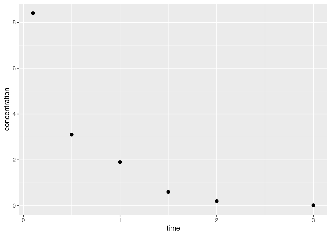
That completes the structural side to our model. Now the statistical side. Again, we’ll keep it simple: I’m going to assume independent and identically normally distributed errors, no matter how unlikely that is in real life. Reflecting the fact that from a statistics point of view we’re now talking about a discrete set of time points and discrete set of measured drug concentrations, I’ll refer to the \(n\) time points as \(t_1, t_2, \ldots, t_n\) and the corresponding observed concentrations as \(c_1, c_2, \ldots, c_n\). In this notation our statistical model is expressed:
\[
c_i = c_0 \ e^{-kt_i} + \epsilon_i
\]
where
\[
\epsilon_i \sim \mbox{Normal}(0, \sigma)
\]
Our model therefore has two unknowns, the scale parameter \(\sigma\) and the elimination rate constant parameter \(k\). Since we are being Bayesians for the purposes of this post I’ll place some priors over these parameters. However, since we are also being lazy Bayesians for the purposes of this post I’m not even going to pretend I’ve thought much about these priors. I’ve made them up because my actual goal here is to familiarise myself with the mechanics of pharmacokinetic modelling in Stan. The real world practicalities – critically important though they are – can wait!
Again, I cannot stress this enough: I literally did not think at all about these choices. Never ever adopt such an appalling practice in real life, boys and girls and enby kids!
It’s almost time to move onto the implementation but first… I kind of lied. There’s a third unknown. The initial concentration \(c_0\) is technically an unknown as well. True, we usually know the dosage to a high degree of precision (if I administer 50μg of a drug, there’s not much error there…), but the volume of the volume of systemic distribution is likely an estimate based on the assumption that blood volume is about 7-8% of body mass. I might guess that this value is about 5.5l but it might be a little more or a little less than that. Allowing the model to have a prior over the true value of \(v_d\) makes some intuitive sense and also has the nice consequence of allowing the model to infer the value of \(c_0\) from the data. In practice we’re not likely to be far wrong in guessing this quantity, so I’ve used the following prior:
\[
v_d \sim \mbox{Normal}(5.5, 1)
\]
where 5.5l is my prior estimate.
Implementation in Stan
Moving along, let’s have a look at how this model would be implemented in Stan. The code for the model is shown below, and – in case you’re not familiar with Stan code – I’ll quickly outline the structure. Stan is a declarative language, not an imperative one: you specify the model, it takes care of the inference. Your code is an abstract description of the model, not a sequence of instructions. In my code below, you can see it’s organised into three blocks:
The data block defines quantities that the user needs to supply. Some of those correspond to empirical data like concentrations, others are design variables for the study like measurement times.
The parameters block defines quantities over which inference must be performed. In this case that’s \(k\) and \(\sigma\).
The model block specifies the model itself, which in this case includes both the structural and statistical components to our model, and does not distinguish between “likelihood” and “prior”. From the Stan point of view Bayesian inference it’s not really about “priors and likelihood” it’s more of a Doctor Who style “modelly-wobbelly joint probability distribution” kind of thing.
Stan is strongly typed with (for example) int and real scalar types, and vector types containing multiple reals.
Variable declarations allow you to specify lower and upper allowable values for variables. It is always good to include those if you know them.
There’s some fanciness going on under the hood in how Stan “thinks about” probability distributions in terms of log-probability functions, but I’m glossing over that because Now Is Not The Time.
I’ve set my lower bounds on the parameters to “something very close to zero” rather than actually zero because (a) those values are wildly implausible anyway, but (b) if the sampler tries to get too close to zero the log probability goes batshit and numerical chaos ensues.
Perhaps more important from the perspective of this post, here’s the important bit of quarto syntax I used when defining the code chunk above. When I defined the code chunk I specified the output.var option by including the following line in the yaml header to the chunk:
#| output.var: "bolus"
By specifying output.var: "bolus" I’ve ensured that when the quarto document is rendered there is a model object called bolus available in the R session. It’s essentially equivalent to having the code above saved to a file called bolus.stan and then calling the cmdstanr function cmdstan_model() to compile it to C++ with the assistance of Stan:
bolus <-cmdstan_model("bolus.stan")
For future Stan models I’ll just print the name of the output variable at the top of the code chunk so that you can tell which R variable corresponds to which Stan model.
In any case let’s take a look at our bolus object. Printing the object yields sensible, if not exciting, output: it shows you the source code for the underlying model:
Perhaps more helpfully for our purposes, it’s useful to know that this is an object of class CmdStanModel, and if you take a look at the documentation on the linked page, you’ll find a description of the methods available for such objects. There are quite a few possibilities, but a few of particular interest from a statistical perspective are:8
$sample() calls the posterior sampling method implemented by Stan on the model
$variational() calls the variational Bayes algorithms implemented by Stan on the model
For the purposes of this post I’ll use the $sample() method, and in order to call it on my bolus object I’ll need to specify some data to pass from R to the compiled Stan model. These are passed as a list:
Delightful, truly. So neat. So clean. So obviously, obviously fictitious.
As a Bayesian9 that has observed the data, what I want to compute is the joint posterior distribution over my parameters \(k\) and \(\sigma\). Or, since this has been an unrealistic expectation ever since the death of the cult of conjugacy,10 what I’ll settle for are samples from that joint posterior that I can use to numerically estimate whatever it is that I’m interested in. To do this for our bolus model with the help of cmdstanr, we call bolus$sample():
This is an object of class CmdStanMCMC and again you can look at the linked page to see what methods are defined for it. I’ll keep things simple for now and call the $summary() method, which returns a tibble containing summary statistics associated with the MCMC chains:
Evidently the estimated posterior mean for the elimination rate constant \(k\) is 2.09, with a 90% credible interval1112 of [1.6, 2.71]. Similarly, the standard deviation of the measurement error \(\sigma\) is estimated to have mean 0.56 and 90% interval [0.29, 1.02].
If we wanted to we could take this a little further by pulling out the posterior samples themselves using the $draws() method. Internally this method relies on the posterior package, and supports any of the output formats allowed by that package. In this case I’ll have it return a tibble because I like tibbles:
You could then go on to do whatever you like with these samples but I have other fish to fry so I’m going to move on.
Generated quantities
The model I built in the previous section is perfectly fine, as far as it goes, but it’s missing something that matters a lot to me. There’s nothing in the code that allows me to use the inferred model parameters to make predictions about the shape of the concentration-time curve across the full range of times. To do that I’ll introduce a “generated quantities” block to my code, as shown below:
When I do this, the data that I pass to this version of the model needs to be modified too. It needs to specify the times for which we want to generate fitted curves:
Warning: 3 of 4000 (0.0%) transitions ended with a divergence.
See https://mc-stan.org/misc/warnings for details.
The bolus2_fitted object contains both the parameter values sampled during the MCMC routine, and the generated quantities that emerged in the process. If I wanted to I could use those generated quantities as is. However, because there’s some value in separating the “posterior prediction” process from the “posterior sampling” process, it’s generally considered best practice to create a new set of generated quantities sampled using the posterior parameter distribution. We can do that by calling the $generate_quantities() method of our fitted model object:
Running standalone generated quantities after 4 MCMC chains, 1 chain at a time ...

Chain 1 finished in 0.0 seconds.
Chain 2 finished in 0.0 seconds.
Chain 3 finished in 0.0 seconds.
Chain 4 finished in 0.0 seconds.

All 4 chains finished successfully.
Mean chain execution time: 0.0 seconds.
Total execution time: 0.5 seconds.
This is a CmdStanGQ object, and again it has $draws() and $summary() methods. For our purposes the $summary() method will suffice as it returns a tibble containing the thing I want to plot:
Having done so I can now draw the plot I really want:
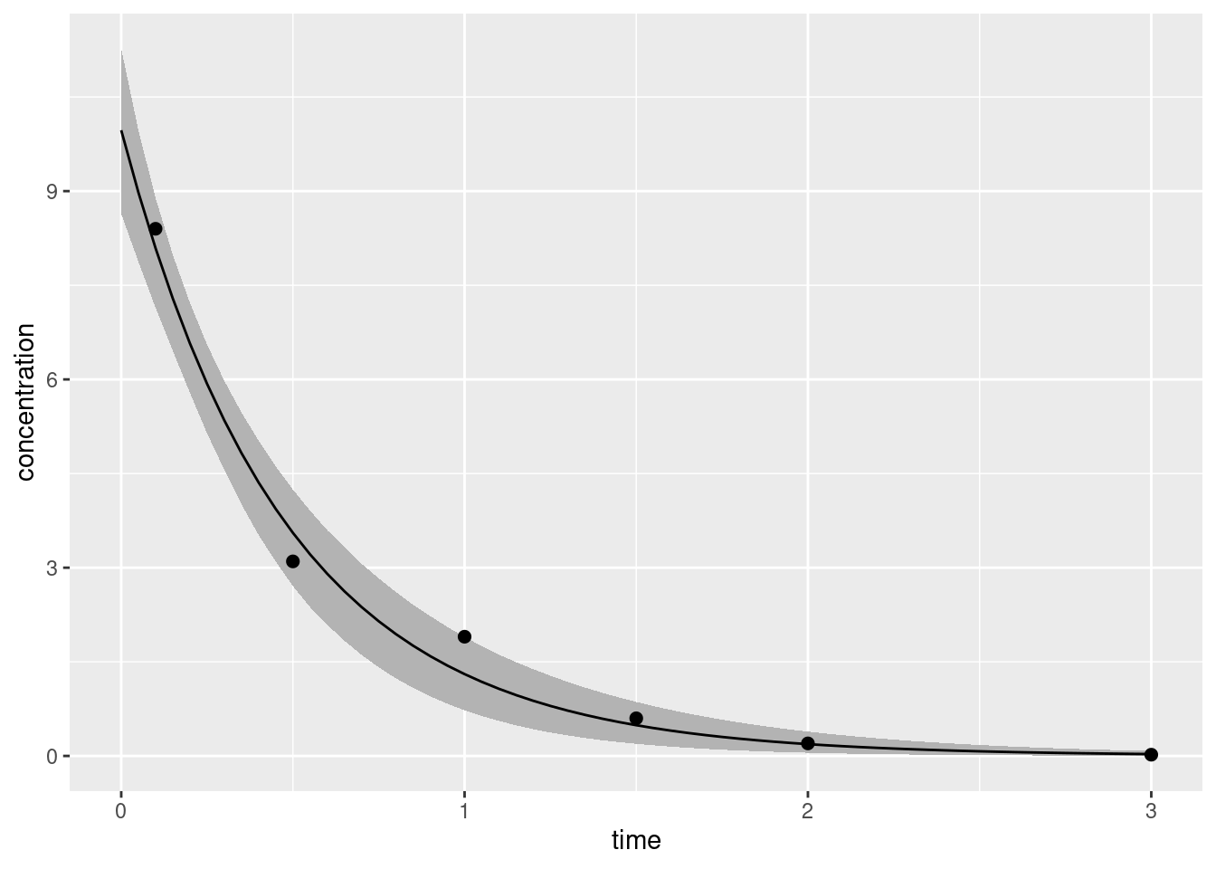
df <-data.frame(t_obs = bolus2_data$t_obs, c_obs = bolus2_data$c_obs)ggplot(bolus2_summary) +geom_ribbon(aes(time, ymin = q5, ymax = q95), fill ="grey70") +geom_line(aes(time, mean)) +geom_point(aes(t_obs, c_obs), data = df, size =2) +labs(x ="time", y ="concentration")
The solid line gives our best point estimate of the true concentration-time curve, and the shaded region shows a 90% credible interval that expresses our uncertainty about what part of the space the true curve might actually occupy.13
I think this is my very favourite piece from this system. The texturing worked out so well.
When biology isn’t analytically tractable
Earlier when I justified the use of an exponential concentration-time function \(C(t)\), I did so by assuming that the body is able to “clear” a constant volume of blood per unit time. That assumption works reasonably well in some situations. If we suppose that the kidneys14 work a bit like a filter, you can imagine that the body is filtering the blood at a fixed rate, which produces the exponential curve I used earlier. But the real world is a little more complicated than that sometimes.
Suppose, instead, that the elimination process involves an enzyme-catalysed reaction. That is, the body eliminates the drug (the substrate) by binding it to enzyme, and from this transition state it is catalysed to something else (the product). The dynamics of such a process are a little different: the enzyme concentration is often very low relative to the substrate concentration and the reaction rate saturates: once you’ve hit that point adding more of the drug into the blood won’t speed up the rate of elimination because there’s no free enzyme to catalyse its conversion. Put slightly differently, if elimination involves a saturable process it won’t necessarily have a constant clearance rate, and you won’t see an exponential concentration-time function.
Well, that’s awkward.
Michaelis-Menten kinetics
The paper I’ve relied on for an introduction to compartmental models in pharmacometrics is Holz and Fahr (2001) and they use Michaelis-Menten kinetics as an example of a saturable elimination process. Michaelis-Menten kinetics is characterised by the following differential equation:
In this expression, \(v_{m}\) is a constant that denoting the maximum velocity of elimination: due to the limitations imposed by the enzyme concentration, the drug concentration cannot decrease faster than this rate. The term \(k_m\) is the Michaelis constant: when the drug concentration \(C(t)\) equals \(k_m\), the elimination rate \(\frac{dC(t)}{dt}\) is exactly half its maximum rate, \(\frac{v_m}{2}\). Both of these properties are easy enough to demonstrate if you’re willing to spend a few minutes playing around with the equation above, but it’s not very interesting, so we’ll move on. A more useful approach is to think about how we should expect Michaelis-Menten kinetics to behave at high and low drug concentrations:
If the drug concentration \(C(t)\) is very large, \(\frac{dC(t)}{dt}\) will be roughly constant and very close to the satuation rate \(v_m\). In other words: At high concentrations, the concentration decreases linearly over time.
If the drug concentration \(C(t)\) is very small, then \(\frac{v_m}{k_m + C(t)}\) will be roughly constant, and \(\frac{dC(t)}{dt}\) will be roughly proportional to the concentration \(C(t)\). In other words: At low concentrations the concentration decreases exponentially over time.
Now that we have a sensible intuition, we should try to draw the actual curves. One teeny-tiny problem… this differential equation doesn’t really have an analytic solution.15 We’re going to have to do this numerically.
What does it look like?
In a moment I’m going to implement Michaelis-Menten kinetics using Stan, so as to eventually give me the ability to do Bayesian statistics in a pharmacokinetic model that involves this kind of dynamics. However, I’m a big fan of doing things in small steps. For example, if I weren’t planning to build all this into a probabilistic model, I wouldn’t really need to use Stan at all. R has many different tools for solving differential equations numerically, and I could just use one of those.
For instance, if I chose to use the deSolve package, I’d begin by defining an R function mmk() that returns the value of the derivative at a given point in time and given specified parameters, pass it to the ode() solver supplied by deSolve, and then draw myself a pretty little picture using ggplot2:
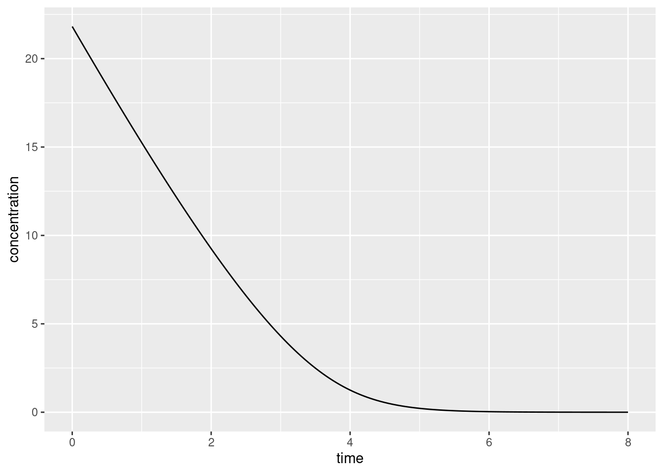
library(deSolve)library(ggplot2)# differential equation for MM kinetics: it returns a list because# that's what ode() expects to receive when it calls this functionmmk <-function(t, y, parms) { dydt <-- y * parms["vm"] / (parms["km"] + y) return(list(dydt))}# parametersdose <-120# (in milligrams)circulation_vol <-5.5# (in litres)max_elimination <-8halving_point <-4times <-seq(0, 8, .05) # (in hours)# use the desolve packageout <-ode(y =c("conc"= dose/circulation_vol),times = times,func = mmk,parms =c("vm"= max_elimination, "km"= halving_point ))# convert matrix to tibble and plotout <-as.data.frame(out)ggplot(out, aes(time, conc)) +geom_line() +labs(x ="time", y ="concentration")
Consistent with the intuitions we developed earlier you can see that on the left hand side this curve looks pretty linear, but on the right hand side it looks pretty much like an exponential decay.
The exact same thing, but in Stan this time
Having solved the relevant differential equation in R, it’s helpful – if slightly strange – to imagine solving the exact same problem using Stan. Although Stan is primarily a language for probabilistic inference, it does provide a toolkit for solving differential equations. In normal usage we’d use the Stan ODE solver in the context of a larger statistical model, but – in order to wrap my head around how it works – I found it helpful to try invoking the solver for a dynamical system without incorporating it into any statistical model.
So let’s do that for Michaelis-Menten kinetics. If we squint and ignore the details, the basic idea is the same in Stan as it was in the earlier example in R:
Write a user-defined function called mmk() that takes arguments for the time, current state of the system (in our case concentration), and any other parameters (the maximum elimination rate and the Michaelis constant), and returns the derivatives.
Call the ODE solver function, in this case ode_rk45(), passing it the user-defined function and other required quantities. This being Stan, we’ll need to ensure those quantities are defined in the data block.
The actual code is shown below. The function is defined within the functions code block (shocking, right?), input data defined within the data block, and the variable we’re trying to compute (conc) is defined as a generated quantity:
It may seem strange that the mmk() function defines the state variable to be a vector of length 1. At first pass it might seem a lot simpler to specify a scalar real: if we did that, then we wouldn’t have the weirdness of defining conc as a one-dimensional length nt array, in which each cell is a vector of length 1, each of which contains a single real number. The layers of nesting seem unnecessary.
However, they are entirely necessary.
To see this, it’s important to recognise that mmk() isn’t an arbitrary user defined function, it is the ODE system function and is designed to be passed to one of the solvers, in this case ode_rk45(). In this particular case our state is one-dimensional: we have a one-compartment model, and the only variable that defines the state is the drug concentration in that compartment. But dynamical systems can be – and usually are – multivariate: in a two-compartment model the state would probably be defined in terms of two drug concentrations, one for each compartment. In that case we would require a vector.
To accommodate this cleanly, the design choice made in Stan is that the second argument to the system function must be a vector, even if the state happens to be one-dimensional. More generally, the point I’m making here is that to call the ODE solvers you need to ensure that your system function has the appropriate signature.
In any case, let’s take our code for a spin. First we’ll create some data that we can pass to Stan:
times <-seq(.05, 8, .05)mmk_data <-list(c0 =21.8, t0 =0, ts = times, vm =8,km =4,nt =length(times))
Next, we “sample” from the “model”. This step is, admittedly, super weird. We don’t actually have a model, and there are no parameters to sample and there are no probabilistic aspects to the system at all. This is going to be the world’s shortest MCMC run. The Stan model above is available in R via the mmk object, so I’ll call its $sample() method, specifying fixed_param = TRUE so that Stan doesn’t try to resample parameters that don’t exist. I’m only going to run one “chain” for a single iteration, because I only need to solve the system once:
Running MCMC with 1 chain...

Chain 1 Iteration: 1 / 1 [100%]  (Sampling)
Chain 1 finished in 0.0 seconds.
Because Stan has dutifully generated the generated quantities, I now have the values for the solved concentrations. I’ll extract those by calling the $draws() method, do a tiny bit of cleanup to wrangle the data into a nice format…
ggplot(mmk_draws, aes(time, conc)) +geom_line() +labs(x ="time", y ="concentration")
Yup, same as before.
Honestly, I just included this one because it’s weird and I’m a sucker for this palette.
One compartment bolus model with MMK elimination
Some preliminaries. For the purposes of building priors it’s useful to think about what kinds of properties you can have sensible intuitions about. It’s a little tricky to set a joint prior over the maximum elimination rate \(v_m\) and the Michaelis constant \(k_m\) without using some outside knowledge. If the data don’t span a range that lets you unambiguously discover “a linear bit” and “an exponential bit” it’s very easy to trade off one parameter against the other. Increasing \(v_m\) and \(k_m\) at the same time will slightly change the “bendiness” of the curve, but that’s easily absorbed into the error terms. In other words, if you don’t have sensible constraints you’re going to end up with a serious identifiability problem. With that in mind, the two thoughts I had are:
I can see why it would be important to understand \(v_m\) and \(k_m\) theoretically but from a data analysis perspective, I found it a little easier to set priors by thinking about the elimination rate \(v_0\) at time \(t = 0\). After a little high school algebra we obtain the following expressions to transform from \(v_0\) to \(v_m\) and vice versa:
Extending this logic, instead of parameterising the prior in terms of the Michaelis constant \(k_m\) (the concentration at which the reaction rate falls to half its maximum value), we can use a design-specific analog, \(k_0\), denoting the concentration at which the reaction rate falls to half of \(v_0\). Again, some algebraic shenanigans gives us the transformations:
In a sign that I still haven’t really nailed this, the way I’m going to set my priors for the model is kind of unprincipled. I’ll set independent priors over the initial rate \(v_0\), and the Michaelis constant \(k_m\). I suppose I could make a pretense of a justification for this, by saying that the prior over \(v_0\) is used to capture my intutions about the experimental design and the prior over \(k_m\) is used to capture my intuitions about the fundamental biological processes as they exist outside the experiment but… yeah, that’s 100% a post hoc rationalisation. The actual reason I’m doing this is that I tried several different ways of setting a prior, and this version seemed to be the least vulnerable to numerical problems. Other versions tended to move into regions of the space where the ODE solver becomes very unhappy, or regions where the target probability density is not well-behaved. Practicality rules my world.
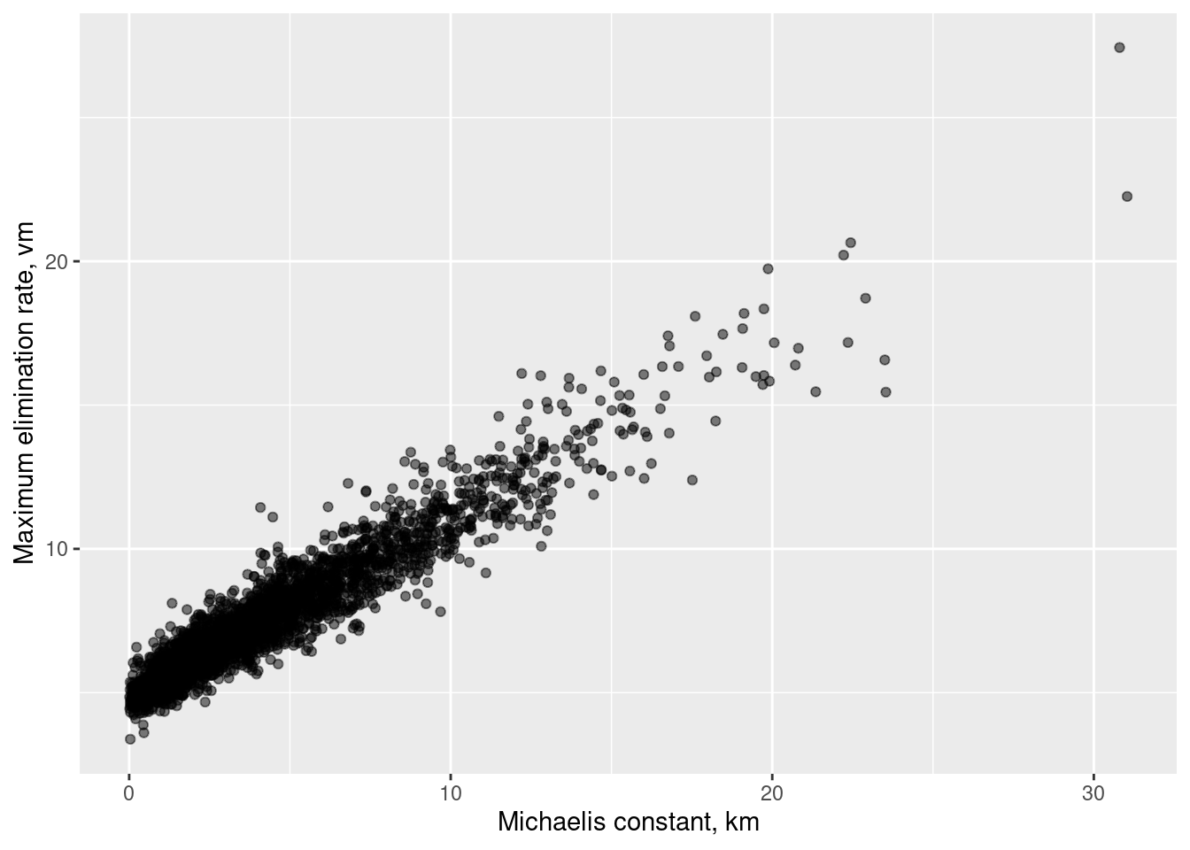
Later, when I plot model posteriors, I’ll be a little more sensible though and use the two interpretable versions: I’ll plot \(v_m\) against \(k_m\), and \(v_0\) against \(k_0\).
The model
Here’s the Stan code for the model I settled on:16
It’s truly thrilling, is it not? You’ll notice that I’ve introduced a “transformed parameters” block in which I’ve define the c0 and vm variables. These are included as transformed parameters because they are quantities that follow deterministically from the “stochastic” parameters (v0, km, etc) and the data, but – unlike the “generated quantities” – they actually do form part of the model because they are used later. The ODE solver needs access to both c0 and vm in order to calculate the model-predicted concentrations at each time point, so they aren’t purely auxiliary. In contrast, the c_fit and k0 variables that I’ve included in the “generated quantities” block aren’t used for anything: the human user (me) wants to know what these values are, but the model doesn’t strictly need them.
And, because human beings typically prefer pretty pictures to tiresome lists of numbers, here’s a plot that shows you what the to-be-modelled data look like:
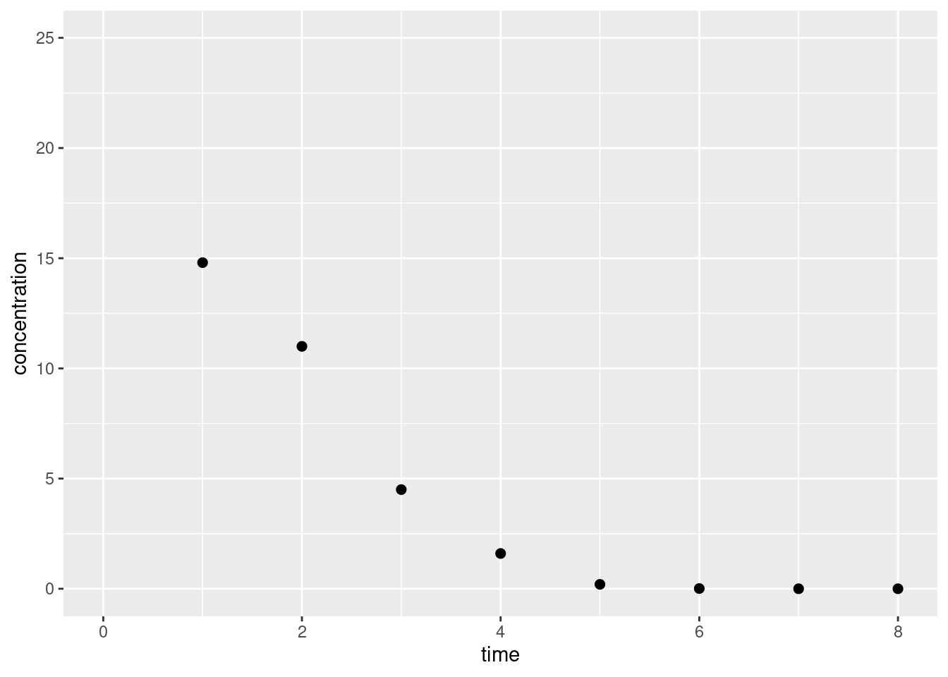
df <-data.frame(time = mmk_bolus_data$t_obs,conc = mmk_bolus_data$c_obs)ggplot(df, aes(time, conc)) +geom_point(size =2) +lims(x =c(0, 8), y =c(0, 25)) +labs(x ="time", y ="concentration")
I kind of like this as a toy data set because it’s (a) very clean, in the sense that it doesn’t feel noisy at all and we expect that the measurement error \(\sigma\) should be pretty small, and (b) there’s just a tiny bit of ambiguity about where precisely the MMK dynamics kick in… looking carefully at these points there’s this feeling that they aren’t really an exponential curve or a linear function, but something in between. So we should be able to model them using a MMK system, but it’s not quite clear where the linear part ends and where the exponential part begins. So it should be instructive…
Okay, let’s take a look at the posterior distributions. As I hinted earlier on – and indeed has been pointed out previously in the literature on Michaelis-Menten kinetics – there is a serious identifiability issue when parameters are expressed in the \((k_m, v_m)\) space:
The very high posterior correlation (the value is 0.96) between \(k_m\) and \(v_m\) makes it nigh-impossible to uniquely identify either one, and I am pretty sure this is also the reason why this particular model is very temperamental. Sure, it looks pretty well behaved in the output above (there are no warning messages and only two divergences reported), but that’s what it looks like after I reparameterised the model into a format that sorta kinda works. The version I implemented originally made Stan cry. A lot.
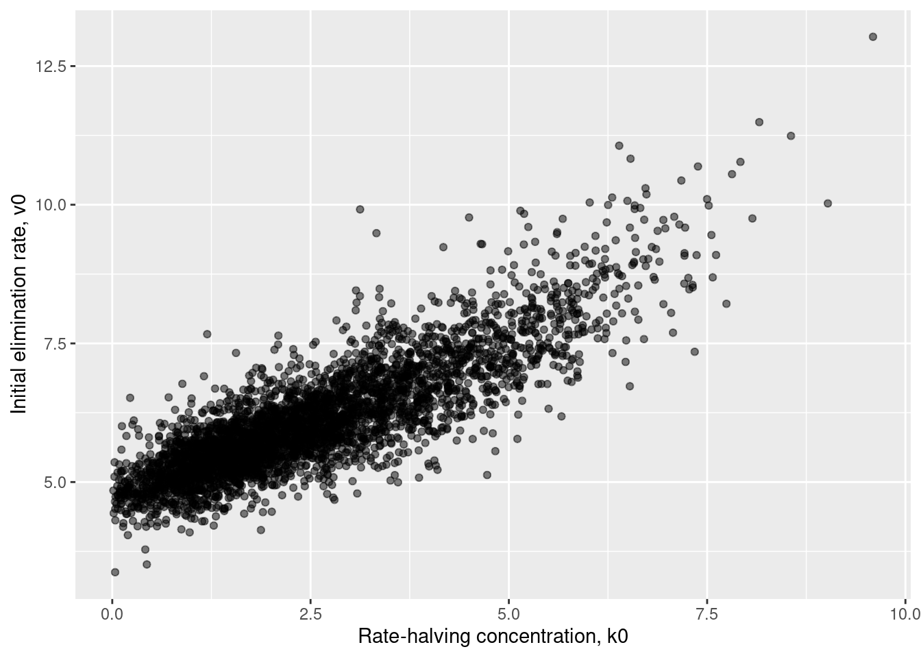
In case you’re interested, here’s what the joint posterior looks like in the \((k_0, v_0)\) space. There’s still some correlation there (the value is 0.85), but it has attenuated quite a bit:
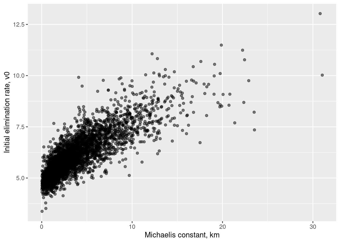
This is the real reason I introduced these transformations! Finally, let’s look at the posterior in the \((k_m, v_0)\) space in which I actually specified my priors:
The correlation here is 0.82, pretty similar to the previous one.18
Credible intervals for the pharamacokinetic function
Okay, let’s turn to the curve itself. While there are some difficulties associated with recovering parameters of the Michaelis-Menten process, the concentration-time curves themselves are pretty recoverable. First, we use our posterior parameters to generate posterior predicted values for the concentration over time:
Running standalone generated quantities after 4 MCMC chains, 1 chain at a time ...

Chain 1 finished in 0.0 seconds.
Chain 2 finished in 0.0 seconds.
Chain 3 finished in 0.0 seconds.
Chain 4 finished in 0.0 seconds.

All 4 chains finished successfully.
Mean chain execution time: 0.0 seconds.
Total execution time: 1.0 seconds.
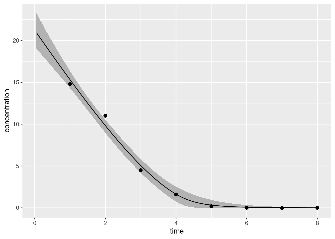
Then we plot the data. The plot below shows the posterior mean estimate of the curve, with the shaded region corresponding to the 90% equal-tail credible intervals for the concentration at each time point. For comparison purposes the observed data are overplotted:
df <-data.frame(t_obs = mmk_bolus_data$t_obs, c_obs = mmk_bolus_data$c_obs)ggplot(mmk_bolus_generated_summary) +geom_ribbon(aes(time, ymin = q5, ymax = q95), fill ="grey70") +geom_line(aes(time, mean)) +geom_point(aes(t_obs, c_obs), data = df, size =2) +labs(x ="time", y ="concentration")
Good enough! Naturally, there’s more I could do with this model, but that’s enough for this post so I’ll move on to something new.
Another favourite of mine. I love the illusion of lighting that you get from the bright bits.
Multi compartment models
Imagine a more complex situation where a drug is administered orally: we now have an influx process where the drug is absorbed from the gut into systemic circulation (the central compartment), from which it is later eliminated. However, if the drug is able to pass between the central compartment and other bodily tissues (the peripheral compartment), we’ll need to model the drug flow between them, since only the drug concentration present in the central compartment is available for potential elimination at any point in time. For the sake of my sanity I’ll assume that it’s just as easy for the drug to pass from central to peripheral as vice versa, so there’s only a single “intercompartmental clearance” parameter associated with this flow. I’m also going to assume that all three processes (absorption, elimination, intercompartmental transfer) involve first order dynamics only.
In this scenario the state at time \(t\) is defined by three concentrations:19
\(c_{gt} = C_g(t)\) is the drug concentration still remaining in the gut
\(c_{ct} = C_c(t)\) is the drug concentration currently in the central compartment
\(c_{pt} = C_p(t)\) is the drug concentration currently in the peripheral compartment
In practice, it can be more convenient to express this in terms of the absolute amount of drug in each compartment (including the gut) at each time point:
\(a_{gt}\) is the drug amount still remaining in the gut
\(a_{ct}\) is the drug amount currently in the central compartment
\(a_{pt}\) is the drug amount currently in the peripheral compartment
where, for each compartment, the concentration is simply the amount divided by the relevant volume, \(c = a /v\). With this in mind we’ll define the state vector at time \(t\) as the three drug amounts, \(\mathbf{a}_t = (a_{gt}, a_{ct}, a_{pt})\).
Strictly speaking, we have four rate parameters in our model:
\(k_a\) is the absorption rate constant (from gut to central compartment)
\(k_e\) is the elimination rate constant from the central compartment
\(k_{cp}\) is the transfer rate from the central to peripheral compartment
\(k_{pc}\) is the transfer rate from the peripheral to central compartment
The biological assumptions of the model are as follows: the gut can only gain drug amount from the external dose which it loses drug to the central compartment, while the peripheral compartment can only exchange drug with the central compartment, and the central compartment has influx from gut, efflux to urine (or whatever), and interchange with the periphery. To help capture this, we’ll define two volumetric parameters:
\(v_c\) is the volume of the central compartment
\(v_p\) is the volume of the peripheral compartment
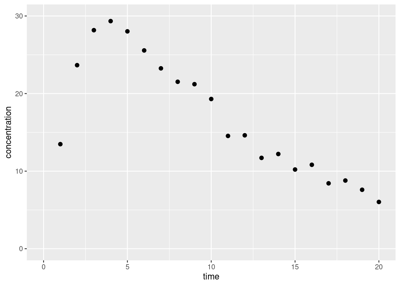
ggplot(obs, aes(t_obs, c_obs)) +geom_point(size =2) +lims(x =c(0, 20), y =c(0, 30)) +labs(x ="time", y ="concentration")
Okay fine yes that looks like data. It’s quite fictitious of course, but whatever. This is a learning exercise for me, not a serious attempt at modelling. Let’s move on, shall we?
Two compartment model
At this point I want to be completely honest. When I started writing this post I really didn’t think I’d reach the point of writing a multi-compartment model. Nevertheless, here we are. On the one hand, I’m pretty pleased with my progress: I set myself a goal and I went well beyond my goal in this post. On the other hand, I am well aware that when I write, I have an audience. So it’s important to recognise that this part of the post is really pushing the boundaries of my current knowledge. Nevertheless, it sorta kinda works. So let’s go with it yeah? This post is long, and we need to finish it somehow. So. Here’s the code:
two_cpt
functions {vector two_cpt(real time,vector state,real qe,real qi,real vc,real vp,real ka) {// convenience...real ag = state[1]; // gut amountreal ac = state[2]; // central amountreal ap = state[3]; // peripheral amount// derivative of state vector with respect to timevector[3] dadt;// compute derivatives dadt[1] = - (ka * ag); dadt[2] = (ka * ag) + (qi / vp) * ap - (qi / vc) * ac - (qe / vc) * ac; dadt[3] = - (qi / vp) * ap + (qi / vc) * ac;return dadt; }}data {int<lower=1> n_obs;int<lower=1> n_fit;vector[n_obs] c_obs;array[n_obs] real t_obs;array[n_fit] real t_fit;vector[3] a0;real t0;}parameters {real<lower=.001> qe;real<lower=.001> qi;real<lower=.001> vc;real<lower=.001> vp;real<lower=.001> ka;real<lower=.001> sigma;}transformed parameters {// use ode solver to find all amounts at all event timesarray[n_obs] vector[3] amount = ode_rk45(two_cpt, a0, t0, t_obs, qe, qi, vc, vp, ka);// vector of central concentrationsvector[n_obs] mu;for (j in1:n_obs) { mu[j] = amount[j, 2] / vc; }}model {// priors (adapted from Margossian et al 2022) qe ~ lognormal(log(10), 0.25); // elimination clearance, CL qi ~ lognormal(log(15), 0.5); // intercompartmental clearance, Q vc ~ lognormal(log(35), 0.25); // central compartment volume vp ~ lognormal(log(105), 0.5); // peripheral compartment volume ka ~ lognormal(log(2.5), 1); // absorption rate constant sigma ~ normal(0, 1); // measurement error// likelihood of observed central concentrations c_obs ~ normal(mu, sigma);}generated quantities {array[n_fit] vector[3] amt_fit = ode_rk45(two_cpt, a0, t0, t_fit, qe, qi, vc, vp, ka);vector[n_fit] c_fit;for (j in1:n_fit) { c_fit[j] = amt_fit[j, 2] / vc; }}
Next, we put together a Stan-friendly version of the data, which includes the initial amount of drug a0 in each compartment (gut, central, peripheral):
That’s a little time consuming and makes me suspect that I’ve implemented this poorly.21 Oh well. Perhaps I’ll revisit later. The important thing is that it sorta works. So let’s move on and take a summary:
Running standalone generated quantities after 4 MCMC chains, 1 chain at a time ...

Chain 1 finished in 0.0 seconds.
Chain 2 finished in 0.0 seconds.
Chain 3 finished in 0.0 seconds.
Chain 4 finished in 0.0 seconds.

All 4 chains finished successfully.
Mean chain execution time: 0.0 seconds.
Total execution time: 2.3 seconds.
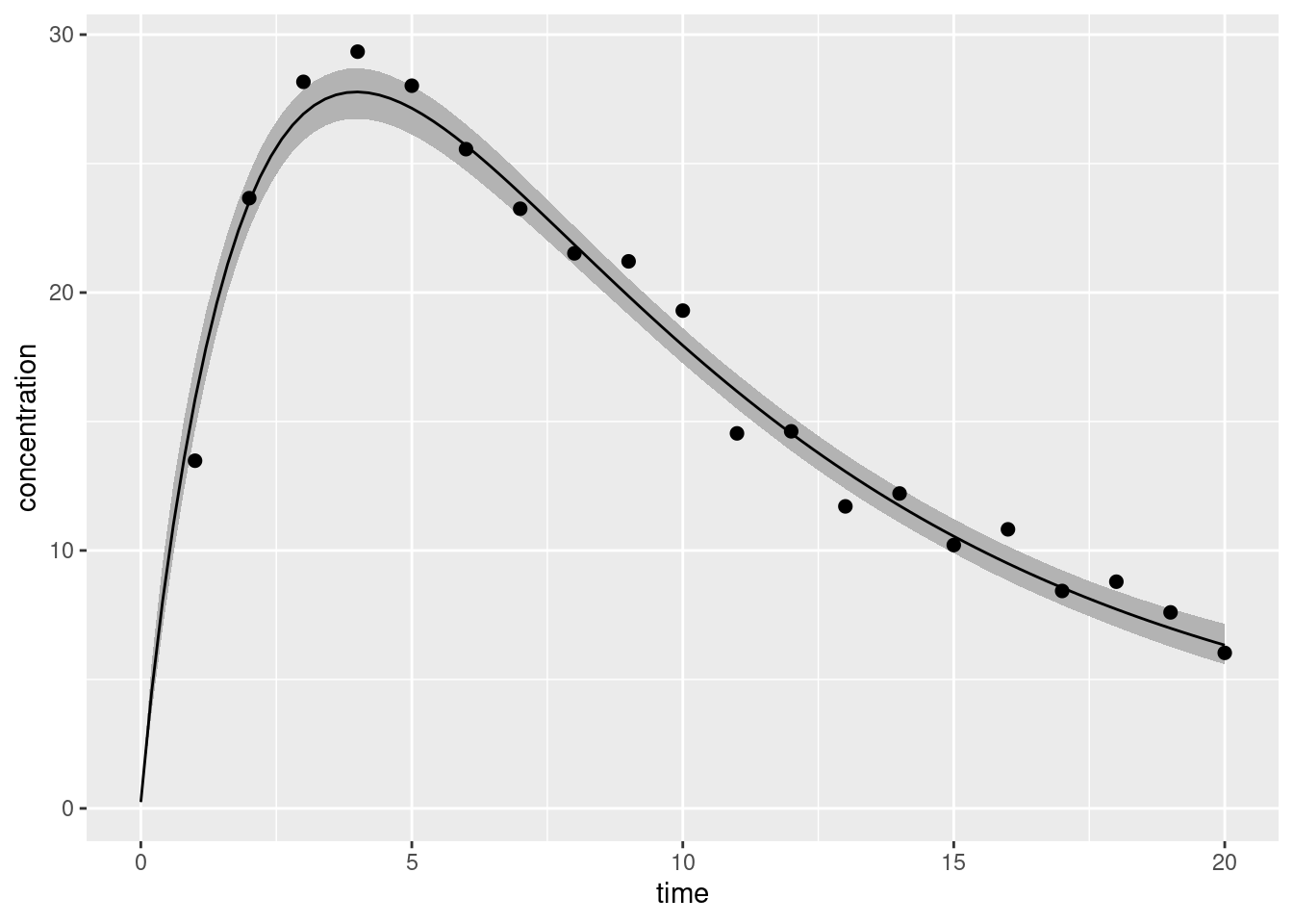
df <-data.frame(t_obs = two_cpt_data$t_obs, c_obs = two_cpt_data$c_obs)ggplot(two_cpt_generated_summary) +geom_ribbon(aes(time, ymin = q5, ymax = q95), fill ="grey70") +geom_line(aes(time, mean)) +geom_point(aes(t_obs, c_obs), data = df, size =2) +labs(x ="time", y ="concentration")
That’s good enough for today.
It’s probably obvious from the context that this is a work in progress. I haven’t really thought this stuff through yet, and I’m willing to put a lot of money on the proposition this code could be improved considerably. However, that’s quite beside the point for this post. Right now, my goal was to get something to work, and this kinda works. Yay! I am happy.
The original system these were based on was called “dreamlike”: the feeling of dissolution in this piece is very characteristic of that ancestor system.
Things I have not discussed
There are many topics that are adjacent to and highly relevant to this post that I have not discussed. The real reason for this is simply that I have limits, and this is just a blog post. But for the sake of listing some of them, here are a few issues around statistical inference that I omitted:
MCMC diagnostics: At various points in the process of writing this post Stan was kind enough to yell very loudly at me about the possibility that things might be going wrong with the MCMC sampler. Having “earned my bones” by writing some truly terrible MCMC samplers of my own, I really appreciate the “fail loudly” aesthetic that Stan has going on. Indeed, the only reason that the models I’ve used here have ended up being… look, let’s call them “okay”, shall we?… is that every time something went awry Stan screamed at me.
Different kinds of ODE solvers: Throughout the post I’ve used ode_rk45() as my ODE solver in Stan, as if that were the only possible choice. It isn’t the only choice, and indeed it’s not even the only solver I used in the process of writing the bloody thing. There were periods in the post development where I couldn’t get the models to behave, and as a consequence of that the sampler kept proposing parameters that pushed the differential equations into a part of the space where they… aren’t pleasant. When that happened the system became “stiff”22 and I had to switch to using ode_bdf(). There is probably a whole blog post to be written about stiffness but… yeah nah. Suffice it to say this is one of those things where the mapmaker feels an urge to scribble “here be dragons” and move along.
Model checking, and Bayesian workflow more generally: Stating the obvious really, but at no point have I really dived into model checking, model testing, etc. There’s a huge amount that could be said on that. Not gonna say any of it here.
There are other things missing too. On the pharmacometric side, I have not discussed:
The logic for choosing one model structure over another. When do you need multiple compartments? When do you need to assume saturating elimination processes? Etc. There’s a very good reason I haven’t spoken about those things: I am not even slightly qualified to do so. That’s something that requires substantive domain knowledge and I’m not there yet.
Individual differences (i.e., population pharmacokinetics). In real life you really need to consider variability across people. That’s something we can address with hierarchical models, by assuming the population defines distributions over parameters. I omitted that for simplicity: I’ll get to that later.
Covariates. Another super important thing in real life is modelling systematic variation across individuals as well as random variation. Predicting the way in which parameters of the process vary across people as a function of other measured characteristics (age, sex, etc) matters hugely. Again, that’s a future topic.
Modelling the effect of the drug (pharmacodynamics): there’s more to these models than simply tracking the drug concentration. Often you need to consider downstream effects… what does the drug do physiologically, or psychologically, and how do those effects persist over time. Future topic babes.
Finally, there are things I’ve missed on the software side. I’ve not talked about Torsten and WinNonlin, and at some point I probably should. But… not today. This post is long enough already. I think we can all agree on that!
Resources
In my post-academic era I’ve gotten a little lax in my citation habits, but I still care about acknowledging my sources. In addition to the various Wikipedia pages and Stan documentation pages I’ve linked to throughout, this blog post draws heavily on ideas presented in these three papers:
Choi, Rempala & King (2017). Beyond the Michaelis-Menten equation: Accurate and efficient estimation of enzyme kinetic parameters. Scientific Reports. doi.org/10.1038/s41598-017-17072-z
Margossian, Zhang & Gillespie (2022). Flexible and efficient Bayesian pharmacometrics modeling using Stan and Torsten, Part I. CPT: Pharmacometrics & Systems Pharmacology. doi.org/10.1002/psp4.12812
Naturally, all the stuff ups and errors are mine and mine alone.
Footnotes
I did try WinBUGS briefly but it was a bit awkward since I wasn’t a Windows user even then.↩︎
Yes, I know that sometimes there are tricks to work around them. It was more effort than it was worth.↩︎
There’s also many packages for specific modelling frameworks like brms and rstanarm but for the purposes of this post I’m only interested in packages that supply a general-purpose interface to Stan from R.↩︎
I mean, technically the real work of compiling the Stan code into an executable and then running the sampler is all being done by Stan itself and has sweet fuck all to do with any R package, but knitr has no way of talking to Stan, so it has to rely on an R package to do that… and by default it asks RStan.↩︎
Or, to those of us who don’t speak the language, the drug is injected into the bloodstream in a single dose.↩︎
Not quite the same as the total amount of blood plasma, as I understand it, but approximately the same idea.↩︎
I’m adopting the $method() convention here sometimes used when discussing R6 classes to be clear that we’re talking about encapsulated OOP in which methods belong to objects (as is typical in many programming languages) rather than functional OOP in which methods belong to generic functions (as appears in the S3 and S4 systems in R, for instance).↩︎
Note for young people: This was the pre-2023 equivalent of saying “As an AI language model…”↩︎
I can still remember quite viscerally the moment that conjugacy died for me as a potentially useful statistical guideline: it was the day I learned that a Dirichlet Process prior is conjugate to i.i.d. sampling from an arbitrary(ish) unknown distribution. DP priors are… well, I don’t want to say “worthless” because I try to see the good in things, but having worked with them a lot over the years I am yet to discover a situation where the thing I actually want is a Dirichlet Process. It’s one of those interesting inductive cases about the projectibility of different properties. What “should” have happened is that the DP-conjugacy property made me more willing to use the DP. Instead, what “actually” happened is that learning about DP-conjugacy made me less willing to trust conjugacy. I knew in my bones that the DP was useless, so I revised my belief about conjugacy. Someone really should come up with a formal language to describe this kind of belief revision… I imagine it would be quite handy.↩︎
This is “of course” (see next footnote) an equal-tailed interval rather than a highest density interval.↩︎
In technical writing, the term “of course” is an expression that used to denote “something that the author is painfully aware of and some subset of the readership is equally exhausted with, and none of those people really want to talk or hear about for the rest of their living days, but is entirely unknown and a source of total confusion to another subset of the readership who have no idea why this should be obvious because in truth it absolutely is not obvious”. As such it should, of course, be used with caution and with a healthy dose of self-deprecation and rolling-of-the-eyes. It is in this latter spirit that my use of the term is intended: I simply do not wish to devote any more of my life to thinking about the different kinds of credible intervals.↩︎
We could supplement it further and maybe add dotted lines even further out that show 90% credible regions for future data (i.e., acknowledging the role of measurement error in the future) but today I don’t feel like doing that!↩︎
And other organs, I guess. I’ve heard rumours the human body contains other organs that actually do things…↩︎
Apparently this is only half true. A deep dive on the relevant wikipedia page suggests that it is possible to solve it analytically, but insofar as the solution involves the Lambert W function I personally would prefer to take a numerical approach.↩︎
Folks familiar with Stan will probably notice that my code style could be improved a little. It’s probably not ideal that I’m enforcing the truncation range on some of my variables twice, once at variable declaration using the <lower, upper> syntax, and then sometimes later on by truncating a distribution using the T[L, U] syntax. At the moment I find this redundancy helpful to me because it stops me from getting confused (e.g., it means I never look at my own code and wonder why my half-normal is declared to have a normal() distribution), but in the long run I think it’s a bad idea for code maintenance. From that point of view I think it makes sense to have a consistent code style that declares variable bounds once and only once, in a place where future maintainers would expect to find it. That would make it a lot easier to edit later. But that’s the kind of detail I’m not going to worry about right this second.↩︎
Okay look, if this were linear regression I’d be very worried at seeing any divergences. But for this model? Babe, this is really fucking good. It took a lot of effort to find a parameterisation of the MMK elimination model that doesn’t end in nuclear fire, metaphorically speaking. One or two divergences in the MCMC chains, yeah, I can live with that.↩︎
Looking at that plot I had wondered if the correlation was being boosted by a few outliers, but that doesn’t seem to be the case: the rank-order correlation for the third plot is 0.82, which compares to 0.83 for the previous plot, and 0.93 for the first one.↩︎
It should be noted that my notation is slightly nonstandard. My understanding is that the convention in the literature is to use notation consistent with the WinNonlin software package, as that is generally considered the industry standard and often used for benchmarking purposes. I haven’t done this for a very boring reason: I’ve not yet had a chance to play around with WinNonlin.↩︎
Again, I know my notation is nonstandard. But I’m still wrapping my head around all this and, for the time being at least, I like having notation that makes clear that \(q_e\) and \(q_{cp}\) are both parameters of the same structural kind. I don’t find CL and Q anywhere near as easy to understand.↩︎
Okay, I should be honest. The real reason I suspect there’s room for improvement here is that I’ve had use show_messages = FALSE to suppress some warnings messages in order to keep the output visually tidy. It’s not terrible: Stan throws some warnings from the ODE solver, especially during the very early stages of warmup, in which it quite rightly screams about being fed insane parameters. It’s not ideal, but it’s not terrible either. I hid the messages to avoid ugly output, not for more nefarious reasons. I mean, don’t get me wrong, this model needs a lot more love than I have given it up to this point. But the hidden warning messages are somewhat boring in this instance.↩︎