

Manuals for translating one language into another can be set up in divergent ways, all compatible with the totality of speech dispositions, yet incompatible with one another
– William Van Orman Quine, 1960, Word and Object
At the 2018 useR! conference in Brisbane, Roger Peng gave a fabulous keynote talk on teaching R to new users in which he provided an overview of the history of the language and how it is used in the broader community. One thing that stood out to me in his talk – and I’ve seen reflected in other data – is that R is unusual as a language because it’s not designed primarily for programmers. Software engineering practices have now become widespread in the R community, and that’s a good thing. Nevertheless, a very large proportion of the R community don’t have a traditional computer science background – and that’s okay! In fact, given the goals of the language that’s a good thing too.
R is a language designed with a practical goal in mind: it is a tool for statistical programming and data analysis. Because of this design focus, R users tend to care most deeply about the tasks that make up their day to day jobs. Few of us care about the IEEE 754 standard for encoding floating point numbers. R users are not typically interested in the big-endian/little-endian distinction. The purpose of R as a high level statistical programming environment is to abstract away from these things, and to allow users to focus on data cleaning, wrangling, and visualisation. R tries to help you get to your data as easily as possible, build models for your data, report those models reliably, and so on. Because that’s the job.
But.
There’s always a “but”, isn’t there?
One of the huge changes in the data science ecosystem in recent years is the change in scale of our data sets. Data sets can now easily encompass billions of rows, and surpass the ability of your machine (and R) to hold in memory. Another huge change in the ecosystem is the proliferation of tools. Data sets have to be passed from one system to another, and when those data sets are large, problems follow. Apache Arrow solves these problems by providing a multi-language toolbox for data exchange and data analysis. It’s a toolbox designed for a big data environment, and a many-language environment. From the perspective of an R user, it supplies the arrow package that provides an interface to Apache Arrow, and through that package allows you to have access to all the other magic that Arrow exposes. It’s an extremely powerful toolbox… but to use it effectively you do need to learn more of those low-level concepts that we as R users like to skim over.
This post is an attempt to fill that gap for you! It’s a long form post, closer to a full length article than a typical blog. My goals in this post are to:
- Walk you through (some of!) the low level implementation details for basic data types: how R represents an integer or a numeric, or a date/time object, etc
- Discuss how and why Arrow and R sometimes make different choices in these details
- Show you how the arrow package translates between R and Arrow
- Include lots of pretty art, because lets face it, this isn’t an exciting topic!
This post isn’t intended to be read in isolation. It’s the third part of a series I have been writing on Apache Arrow and R, and it probably works best if you’ve read the previous two. I’ve made every effort to make this post self-contained and self-explanatory, but it does assume you’re comfortable in R and have a little bit of knowledge about what the arrow package does. If you’re not at all familiar with arrow, you may find it valuable to read the first post in the series, which is a getting started post, and possibly the second one that talks about the arrow dplyr backend.
Still keen to read? I haven’t scared you off?
No?
Fabulous! Then read on, my loves!
library(tibble)
library(dplyr)
Attaching package: 'dplyr'The following objects are masked from 'package:stats':
filter, lagThe following objects are masked from 'package:base':
intersect, setdiff, setequal, unionlibrary(arrow)
Attaching package: 'arrow'The following object is masked from 'package:utils':
timestampRegarding magic
Consider this piece of magic. I have a csv file storing a data set. I import the data set into R using whatever my favourite csv reader function happens to be:
magicians <- read_csv_arrow("magicians.csv")
magicians
# A tibble: 65 × 6
season episode title air_date rating viewers
<int> <int> <chr> <date> <dbl> <dbl>
1 1 1 Unauthorized Magic 2015-12-16 0.2 0.92
2 1 2 The Source of Magic 2016-01-25 0.4 1.11
3 1 3 Consequences of Advanced Spellcasti… 2016-02-01 0.4 0.9
4 1 4 The World in the Walls 2016-02-08 0.3 0.75
5 1 5 Mendings, Major and Minor 2016-02-15 0.3 0.75
6 1 6 Impractical Applications 2016-02-22 0.3 0.65
7 1 7 The Mayakovsky Circumstance 2016-02-29 0.3 0.7
8 1 8 The Strangled Heart 2016-03-07 0.3 0.67
9 1 9 The Writing Room 2016-03-14 0.3 0.71
10 1 10 Homecoming 2016-03-21 0.3 0.78
# ℹ 55 more rowsThen I decide to “copy the data into Arrow”.1 I do that in a very predictable way using the arrow_table() function supplied by the arrow package:
arrowmagicks <- arrow_table(magicians)
arrowmagicks
Table
65 rows x 6 columns
$season <int32>
$episode <int32>
$title <string>
$air_date <date32[day]>
$rating <double>
$viewers <double>This is exactly the output I should expect, but the longer I think about it the more it seems to me that something quite remarkable is going on. Some magic is in play here, and I want to know how it works.
To understand why I’m so curious, consider the two objects I now have. The magicians data set is a data frame (a tibble, technically) stored in R. The arrowmagicks data set, however, is a pointer to a data structure stored in Arrow. That data structure is a Table object. Table objects in Arrow are roughly analogous to data frames – both represent tabular data with columns that may be of different types – but they are not the same. The columns of a Table are built from objects called ChunkedArrays that are in turn constructed from Arrays, and those Arrays can contain Scalar objects. In other words, to move data from one language to another an act of translation is required, illustrated below:
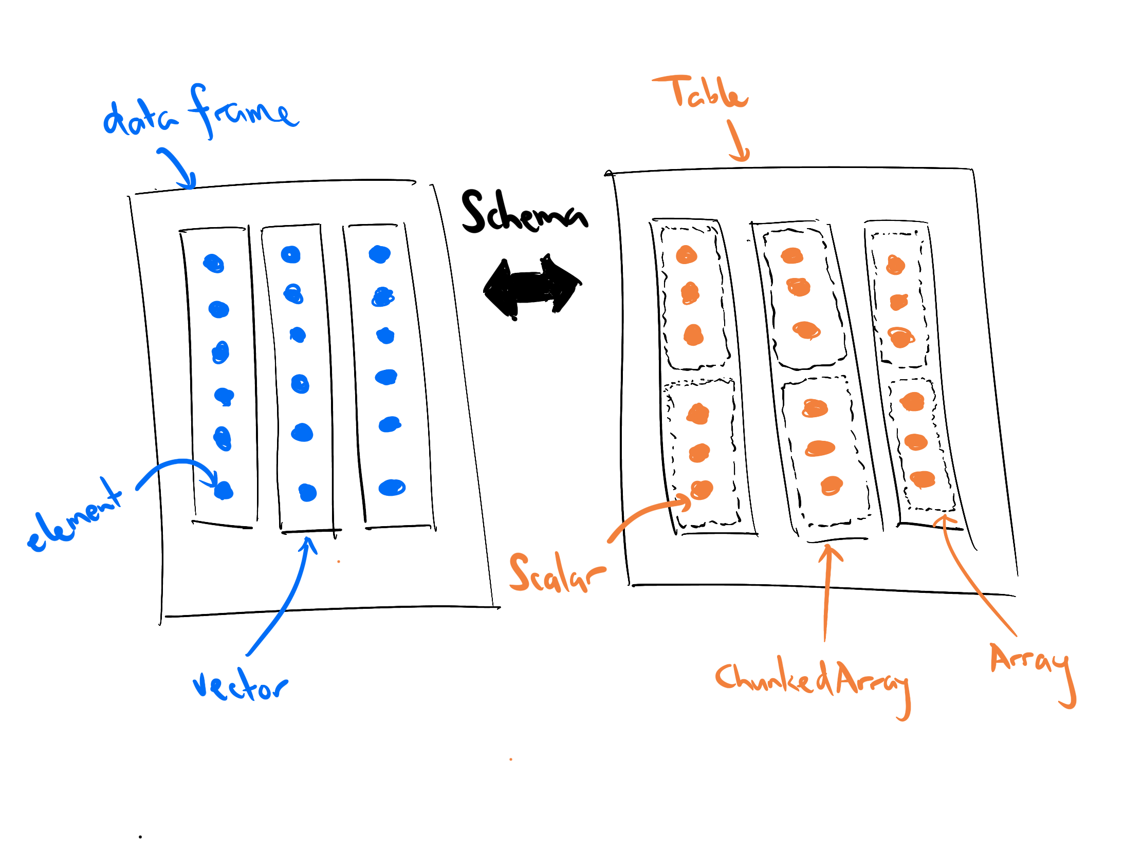
In this post I’m not going to talk much about the difference between Arrays and ChunkedArrays, or why Arrow organises Tables this way (that will be the topic of a later post). For now it’s enough to recognise that Arrow does have this additional structure: the Table data type in Arrow is not equivalent to the data frame class in R, so a little work is required to map one to the other.
A similar story applies when we look at the contents of the data set. The translation process doesn’t just apply to the “container” object (i.e., the data frame in R and the Table in Arrow), it also applies to the values that the object contains. If we look at the how the columns of magicians and arrowmagicks are labelled, we see evidence of this translation. The integer columns in R have been mapped to int32 columns in Arrow, Date columns in R become date32 columns in Arrow, and so on.
There’s quite a lot of complexity to the translation process, yet it all seems to work seamlessly, and it works both ways. I can pull the arrowmagicks data back into R and recover the original data:
collect(arrowmagicks)# A tibble: 65 × 6
season episode title air_date rating viewers
<int> <int> <chr> <date> <dbl> <dbl>
1 1 1 Unauthorized Magic 2015-12-16 0.2 0.92
2 1 2 The Source of Magic 2016-01-25 0.4 1.11
3 1 3 Consequences of Advanced Spellcasti… 2016-02-01 0.4 0.9
4 1 4 The World in the Walls 2016-02-08 0.3 0.75
5 1 5 Mendings, Major and Minor 2016-02-15 0.3 0.75
6 1 6 Impractical Applications 2016-02-22 0.3 0.65
7 1 7 The Mayakovsky Circumstance 2016-02-29 0.3 0.7
8 1 8 The Strangled Heart 2016-03-07 0.3 0.67
9 1 9 The Writing Room 2016-03-14 0.3 0.71
10 1 10 Homecoming 2016-03-21 0.3 0.78
# ℹ 55 more rowsIn this example the translation back and forth “just works”. You really don’t have to think too much about the subtle differences in how Arrow and R “think about the world” and how their data structures are organised. And in general that’s what we want in a multi-language toolbox: we want the data analyst to be thinking about the data, not the cross-linguistic subtleties of the data structures!
That being said, it’s also valuable to give the data analyst flexibility. And that means we’re going to need to talk about Schemas. As shown in the “translation diagram” above, Schemas are the data structure arrow uses to govern the translation between R and Arrow, and since I’m going to be talking about data “on the R side” and data “on the Arrow side” a lot, it will be helpful to have some visual conventions to make it a little clearer. Throughout the post you’ll see diagrams showing the default mappings that the arrow package uses when converting data columns from R to Arrow and vice versa. In each case I’ll show R data types on the left hand side (against a blue background) and Arrow data types on the right hand side (against an orange background), like this:

Defining Schemas
The arrow package makes very sensible default choices about how to translate an R data structure into an Arrow data structure, but those choices can never be more than defaults because of the fundamental fact that the languages are inherently different. The quote about the indeterminacy of translation at the top of this post was originally written about natural languages, but I think it applies in programming too. There’s no single rulebook that tells you how to translate between R and Arrow: there can’t be.2
Suppose that I knew that there would in fact be a “Season 5.1648” coming, consisting of a single episode that would air not only on a specific date, but at a specific time that would – for some bizarre reason3 – be important to encode in the data. Knowing that this new data point is coming, I’d perhaps want my Arrow data to encode season as a numeric variable, and I’d need to encode the air_date field using a date type that implicitly encodes time of day. I can do this with the schema() function:
translation <- schema(
  season = float64(), # not the default
  episode = int32(),
  title = utf8(),
  air_date = date64(), # not the default
  rating = float64(),
  viewers = float64()
)
Now I can use my schema to govern the translation:
arrowmagicks2 <- arrow_table(magicians, schema = translation)
arrowmagicks2
Table
65 rows x 6 columns
$season <double>
$episode <int32>
$title <string>
$air_date <date64[ms]>
$rating <double>
$viewers <double>The output may not make complete sense at this point, but hopefully the gist of what I’ve done should be clear. The season is no longer stored as an integer (it’s now a numeric type), and the air_date no longer uses “day” as the unit of encoding, it uses “ms” (i.e., millisecond). I’ve accomplished my goals. Yay!
This is of course a toy example, as are all the other examples you’ll encounter in this post. But the underlying issues are important ones!

Why mapping languages is hard
Organising the world into concepts (or data structures) is hard.4 We define ontologies that impose order on a chaotic world, but those structures are rarely adequate to describe the world as it is. While doing background research for this post I spent a little time reading various sections from An Essay Towards a Real Character, and a Philosophical Language, a monograph written by John Wilkins in 1668 that makes a valiant (but doomed… oh so doomed) attempt to organise all the categories of things and propose a mechanism by which we could describe them within a single universal language. The classification systems he came up with were… not great. For example, he divided BEASTS into two categories: VIVIPAROUS beasts are those that bear live young, whereas OVIPAROUS beasts are those that lay eggs. The viviparous ones could be subdivided into WHOLE-FOOTED ones and CLOVEN-FOOTED ones. The cloven-footed beasts could be subdivided into those that were RAPACIOUS and those that were not. RAPACIOUS types could be of the CAT-KIND or the DOG-KIND.
Suffice it to say the poor man had never encountered a kangaroo.
The problem with trying to construct universal ontologies is that these things are made by humans, and humans have a perspective that is tied to their own experience and history. As a 17th century English gentleman, Wilkins saw the world in a particular way, and the structure of the language he tried to construct reflected that fact.
I am of course hardly the first person to notice this. In 1952 the Argentinian author Jorge Luis Borges published a wonderful essay called The Analytical Language of John Wilkins that both praises Wilkins’ ambition and then carefully illustrates why it is necessarily doomed to fail. Borges’ essay describes a classification system from an fictitious “Celestial Emporium of Benevolent Knowledge” which carves up the beasts as follows:
In its remote pages it is written that the animals are divided into: (a) belonging to the emperor, (b) embalmed, (c) tame, (d) sucking pigs, (e) sirens, (f) fabulous, (g) stray dogs, (h) included in the present classification, (i) frenzied, (j) innumerable, (k) drawn with a very fine camelhair brush, (l) et cetera, (m) having just broken the water pitcher, (n) that from a long way off look like flies
Now, it’s pretty unlikely that any human language would produce a classification system quite as chaotic as Borges’ fictional example, but the point is well made. Actual classification systems used in different languages and cultures are very different to one another and often feel very alien when translated. It’s a pretty fundamental point, and I think it applies to programming languages too.5 Every language carries with it a set of assumptions and structures that it considers “natural”, and translation across the boundaries between languages is necessarily a tricky business.6
A little bit of big picture
Before we get to “moving data around” part it’s helpful to step back a little and recognise that R and Arrow are designed quite differently. For starters, the libarrow library to which the arrow package provides bindings is written in C++, and C++ is itself a different kind of language than R. And in a sense, that’s actually the natural place to start because it influences a lot of things in the design of arrow.
Object oriented programming in arrow
One of ways in which C++ and R differ is in how each language approaches object oriented programming (OOP). The approach taken in C++ is an encapsulated OOP model that is common to many programming languages: methods belong to objects. Anyone coming from outside R is probably most familiar with this style of OOP.
The approach taken in R is… chaotic. R has several different OOP systems that have different philosophies, and each system has its own strengths and weaknesses.7 The most commonly used system is S3, which is a functional OOP model: methods belong to generic functions like print(). Most R users will be comfortable with S3 because it’s what we see most often. That being said, there are several other systems out there, some of which adopt the more conventional encapsulated OOP paradigm. One of the most popular ones is R6, and it works more like the OOP systems seen in other languages.
The arrow package uses both S3 and R6, but it uses them for quite different things. Whenever arrow does something in an “R-native” way, S3 methods get used a lot. For example, in my earlier post on dplyr bindings for Arrow I talked about how arrow supplies a dplyr engine: this works in part by supplying S3 methods for various dplyr functions that are called whenever a suitable Arrow object gets passed to dplyr. The interface between arrow and dplyr uses S3 because this context is “R like”. However, this isn’t a post about that aspect of arrow, so we won’t need to talk about S3 again in this post.
However, arrow has a second task, which is to interact with libarrow, the Arrow C++ library. Because the data structures there all use encapsulated OOP as is conventional in C++, it is convenient to adhere to those conventions within the arrow package. Whenever arrow has to interact with libarrow, it’s useful to be as “C++ like” as possible, and this in turn means that the interface between arrow and libarrow is accomplished using R6. So we will be seeing R6 objects appear quite often in this post.8
Table, ChunkedArray, and Scalar
You may be wondering what I mean when I say that R6 objects are used to supply the interface between R and Arrow. I’ll try to give some concrete examples. Let’s think about the arrow_table() function. At the start of the post I used this function to translate an R data frame into an Arrow Table, like this:
arrow_table(magicians)This is a natural way of thinking about things in R, but the arrow_table() function doesn’t actually do the work. It’s actually just a wrapper function. Within the arrow package is an R6 class generator object called Table,9 and its job is to create tables, modify tables, and so on. You can create a table by using the create() method for Table. In other words, instead of calling arrow_table() I could have done this:
Table$create(magicians)and I would have ended up with the same result.
The same pattern appears throughout the arrow package. When I used the schema() function earlier, the same pattern was in play. There is an R6 class generator called Schema, and it too has a create() method. I could have accomplished the same thing by calling Schema$create().
I could go on like this for some time. Though I won’t talk about all of them in this post, there are R6 objects for Dataset, RecordBatch, Array, ChunkedArray, Scalar, and more. Each of these provides an interface to a data structure in Arrow, and while you can often solve all your problems without ever interacting with these objects, it’s very handy to know about them and feel comfortable using them. As the post goes on, you’ll see me doing that from time to time.
But enough of that! It’s time to start moving data around…

Logical types
At long last we arrive at the point where I’m talking about the data values themselves, and the simplest kind of data to talk about are those used to represent truth values. In R, these are called logical data and can take on three possible values: TRUE and FALSE are the two truth values, and NA is used to denote missing data.10 In a moment I’ll show you how to directly pass individual values from R to Arrow, but for the moment let’s stick to what we know and pass the data across as part of a tabular data structure. Here’s a tiny tibble, with one column of logical values:
dat <- tibble(values = c(TRUE, FALSE, NA))
dat
# A tibble: 3 × 1
values
<lgl>
1 TRUE
2 FALSE
3 NA We’re going to pass this across to Arrow using arrow_table() but before we do let’s talk about what we expect to happen when the data arrive at the other side.
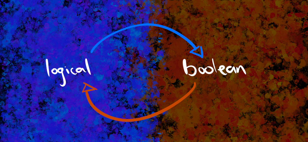
In this case, it’s quite straightforward. Arrow has a boolean type that has truth values true and false that behave the same way as their cousins in R. Just like R, Arrow allows missing values, though they’re called null values in Arrow. Unlike basically every other example we’re going to see in this post, this one is straightforward because the mapping is perfect. Unless you do something to override it, the arrow package will map an R logical to an Arrow boolean and vice versa. Here’s the diagram I use to describe it:
Seems to make sense, right? So let’s stop talking about it and create the corresponding Table in Arrow:
tbl <- arrow_table(dat)
tbl
Table
3 rows x 1 columns
$values <bool>Hm. Okay that’s a little underwhelming as output goes? I’d like to see the actual values please. Happily the arrow package supplies a $ operator for Table objects so we can extract an individual column from tbl the same way we can from the original R object dat. Let’s try that:
tbl$valuesChunkedArray
<bool>
[
[
true,
false,
null
]
]The output looks a little different to what we’d get when printing out a single column of a tibble (or data frame), but it’s pretty clear that we’ve extracted the right thing. A single column inside an Arrow Table is stored as a ChunkedArray, so this looks right.
Yay us!
At this point, it’s handy to remember that the arrow_table() function that I used to move the data into Arrow is really just a wrapper that allows you to access some of the Table functionality without having to think about R6 too much. I also mentioned there’s a class generator called ChunkedArray object and a chunked_array() wrapper function. In hindsight, I probably didn’t need to bother creating the tibble and porting that over as a Table. I could have created a logical vector in R and port that over as a ChunkedArray directly:
values <- c(TRUE, FALSE, NA)
chunked_array(values)
ChunkedArray
<bool>
[
[
true,
false,
null
]
]That’s a cleaner way of doing things. If you want a Table, use Table and its wrappers. If you want a ChunkedArray, use ChunkedArray and its wrappers. There’s no need to over-complicate things.
Speaking of which… later in the post, I’ll often want to send single values to Arrow. In those cases I don’t want to create a ChunkedArray, or even the simpler unchunked Array type. What I want to pass is a Scalar.
It’s worth unpacking this a little. Unlike some languages, R doesn’t really make a strong distinction between “vectors” and “scalars”: an R “scalar” is just a vector of length one. Arrow is stricter, however. A ChunkedArray is a container object with one or more Arrays, and an Array is also a container object with one or more Scalars. If it helps, you can think of it a little bit like working with lists in R: if I have a list lst, then lst[1] is still a list. It doesn’t return the contents of the list. If I want to extract the contents I have to use lst[[1]] to pull them out. Arrow Arrays contain Scalars in a fashion that we would call “list-like” in R.
In any case, the important thing to recognise is that arrow contains a class generator object called Scalar, and it works the same way as the other ones. The one difference is that there aren’t any wrapper functions for Scalar, so I’ll have to use Scalar$create() directly:
Scalar$create(TRUE, type = boolean())Scalar
trueIn this example I didn’t really need to explicitly specify that I wanted to import the data as type = boolean(). The value TRUE is an R logical, and the arrow default is to map logicals onto booleans. I only included it here because I wanted to call attention to the type argument. Any time that you want to import data as a non-default type, you need to specify the type argument. If you look at the list of Apache Arrow data types on the arrow documentation page, you’ll see quite a lot of options. For now, the key thing to note is that the type argument expects you to call one of these functions.
Anyway, that’s everything I had to say about logicals. Before moving on though, I’m going to write my own wrapper function, and define scalar() as an alias for Scalar$create():
scalar <- function(x, type = NULL) {
  Scalar$create(x, type)
}
The main reason I’m doing that is for convenience, because in this post I’m actually going to need this wrapper function a lot. So I should probably check… does it work?
scalar(TRUE)Scalar
trueAwesome!

Integer types
When translating R logicals to Arrow booleans, there aren’t a lot of conceptual difficulties. R has one data structure and Arrow has one data structure, and they’re basically identical. This is easy. Integers, however, are a little trickier because there’s no longer an exact mapping between the two languages. Base R provides one integer type, but Arrow provides eight distinct integer types that it inherits from C++. As a consequence it will no longer be possible to provide one-to-one mappings between R and Arrow, and some choices have to be made. As we’ll see in this section, the arrow package tries very hard to set sensible default choices, and in most cases these will work seamlessly. It’s not something you actually have to think about much. But, as my dear friend Dan Simpson11 reminds me over and over with all things technical, “God is present in the sweeping gestures but the Devil is in the details”.
It is wise to look carefully at the details, so let’s do that.
[Arrow] Eight types of integer
To make sense of the different types, it helps to take a moment to think about how integers are represented in a binary format. Let’s suppose we allocate 8 bits to specify an integer. If we do that, then there are \(2^8 = 256\) unique binary patterns we can create with these bits. Because of this, there is a fundamental constraint: no matter how we choose to set it up, 8-bit integers can only represent 256 distinct numbers. Technically, we could choose any 256 numbers we like, but in practice there are only two schemes used for 8-bit integers: “unsigned” 8-bit integers (uint8) use those bits to represent integers from 0 to 255, whereas “signed” 8-bit integers (int8) can represent integers from -128 to 127.
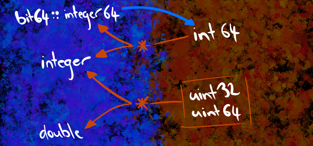
More generally, an unsigned n-bit integer can represent integers from 0 to \(2^n - 1\), whereas a signed n-bit integer can represent integers from \(-2^{n-1}\) to \(2^{n-1} - 1\). Here’s what that looks like for all the integer types supported by Arrow:
| Description | Name | Smallest Value | Largest Value |
|---|---|---|---|
| 8 bit unsigned | uint8 | 0 | 255 |
| 16 bit unsigned | uint16 | 0 | 65535 |
| 32 bit unsigned | uint32 | 0 | 4294967295 |
| 64 bit unsigned | uint64 | 0 | 18446744073709551615 |
| 8 bit signed | int8 | -128 | 127 |
| 16 bit signed | int16 | -32768 | 32767 |
| 32 bit signed | int32 | -2147483648 | 2147483647 |
| 64 bit signed | int64 | -9223372036854775808 | 9223372036854775807 |
[R] One integer class
On the R side, the integer type supplied by base R is a 32 bit signed integer, and has a natural one-to-one mapping to the Arrow int32 type. Because of this, the arrow default is to convert an R integer to an Arrow int32 and vice versa. Here’s an example. I’ve been watching Snowpiercer lately, and the train is currently 1029 cars long so let’s pass the integer 1029L from R over to Arrow
snowpiercer <- scalar(1029L)
snowpiercer
Scalar
1029Let’s inspect the type field of the snowpiercer object in order to determine what type of object has arrived in Arrow:
snowpiercer$typeInt32
int32We can apply the S3 generic function as.vector() to snowpiercer to pull the data back into R,12 and hopefully it comes as no surprise to see that we get the same number back:
as.vector(snowpiercer)[1] 1029We can take this one step further to check that the returned object is actually an R integer by checking its class(), and again there are no surprises:
snowpiercer %>%
  as.vector() %>%
  class()
[1] "integer"As you can see, the default behaviour in arrow is to translate an R integer into an Arrow int32, and vice versa. That part, at least, is not too complicated.
That being said, it’s worth unpacking some of the mechanics of what I’m doing with the code here. Everything I’ve shown above is R code, so it’s important to keep it firmly in mind that when I create the snowpiercer object there are two different things happening: a data object is created inside Arrow, and a pointer to that object is created inside R. The snowpiercer object is that pointer (it’s actually an R6 object). When I called snowpiercer$type in R, the output is telling me that the data object in Arrow has type int32. There’s a division of responsibility between R and Arrow that always needs to be kept in mind.
Now, in this particular example there’s an element of silliness because my data object is so tiny. There was never a good reason to put the data in Arrow, and the only reason I’m doing it here is for explanatory purposes. But in real life (like in the TV shoe), snowpiercer might in fact be a gargantuan monstrosity over which you have perilously little control due to it’s staggering size. In that case it makes a big difference where the data object is stored. Placing the data object in Arrow is a little bit like powering your 1029-car long train using the fictitious perpetual motion engine from the show: it is a really, really good idea when you have gargantuan data.13
When integer translation is easy
What about the other seven C++ integer types? This is where it gets a little trickier. The table above illustrates that some integer types are fully contained within others: unsurprisingly, every number representable by int16 can also be represented by int32, so we can say that the int16 numbers are fully “contained” by (i.e. are a proper subset of) the int32 numbers. Similarly, uint16 is contained by uint32. There are many cases where an unsigned type is contained by a signed type: for instance, int32 contains all the uint16 numbers. However, because the unsigned integers cannot represent negative numbers, the reverse is never true. So we can map out the relationships between the different types like this:
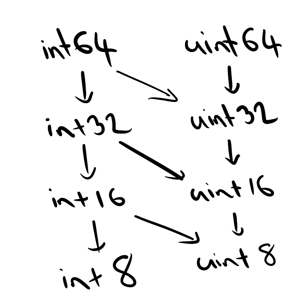
Whenever type A contains type B, it’s possible to transform an object of type B into an object of type A without losing information or requiring any special handling. R integers are 32 bit signed integers, which means it’s possible to convert Arrow data of types int32, int16, int8, uint16, and uint8 to R integers completely painlessly. So for these data types the arrow defaults give us this relationship:
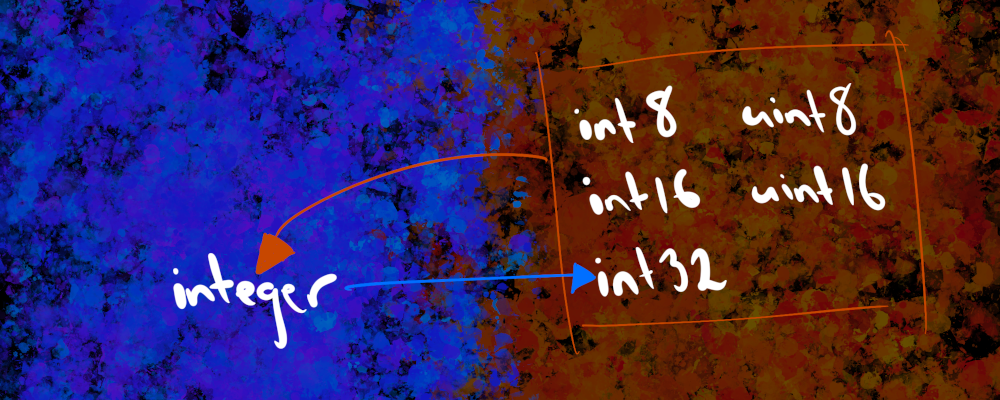
These are the cases where it is easy.
When integer translation is hard
Other integer types are messier. To keep things nice and simple, what we’d like to do is to map the Arrow uint32, uint64, and int64 types onto the R integer type. Sometimes that’s possible: if all the stored values fall within the range of values representable by R integers (i.e., are between -2147483648 and 2147483647) then we can do this, and that’s what arrow does by default. However, if there are values that “overflow” this range, then arrow will import the data as a different type. That leads to a rather messy diagram, I’m afraid:
Translations become messy when the boxes in one language don’t quite match up to the content expressed in another. Sometimes it’s just easier to see the system in action, so let’s write a little helper function:
translate_integer <- function(value, type) {
  fn <- function(value, type) {
    tibble(
      value = value,
      arrow_type = scalar(value, type)$type$name,
      r_class = scalar(value, type) %>% as.vector() %>% class()
    )
  }
  purrr::map2_dfr(value, type, fn)
}
The translate_integer() function takes a value vector and a type list as input, and it returns a tibble that tells you what Arrow type was created from each input, and what R class gets returned when we import that Arrow object back into R. I’ll pass the inputs in as doubles originally, but as you’ll see they always get imported to Arrow as integer types because that’s what I’m telling arrow to do. So let’s start with an easy case. The number 10 is unproblematic because it’s very small, and arrow never encounters any problem trying to pull it back as an R integer:
translate_integer(
  value = c(10, 10, 10, 10),
  type = list(uint8(), uint32(), uint64(), int64())
)
# A tibble: 4 × 3
value arrow_type r_class
<dbl> <chr> <chr>
1 10 uint8 integer
2 10 uint32 integer
3 10 uint64 integer
4 10 int64 integerOkay, that makes sense. If the numbers can be represented using the R integer class then that’s what arrow will do. Why make life unnecessarily difficult for the user?
Now let’s increase the number to a value that is too big to store as a signed 32-bit integer. This is a value that R cannot represent as an integer, but Arrow can store as a uint32, uint64 or int64. What happens when we try to pull that object back into R?
translate_integer(
  value = c(3000000000, 3000000000, 3000000000),
  type = list(uint32(), uint64(), int64())
)
# A tibble: 3 × 3
value arrow_type r_class
<dbl> <chr> <chr>
1 3000000000 uint32 numeric
2 3000000000 uint64 numeric
3 3000000000 int64 integer64The first two rows seem intuitive. In base R, whenever an integer overflows and becomes too large to store, R will coerce it to a double. This is exactly the same behaviour we’d observe if the data had never left R at all. The third row, however, might come as a bit of a surprise. It certainly surprised me the first time I encountered it. Until very recently I did not know that R even had an integer64 class. This class is supplied by the bit64 package, and although I’m not going to talk about it in any detail here, it provides a mechanism to represent signed 64-bit integers in R. However, the one thing I will mention is the fact that the existence of the integer64 class opens up the possibility of forcing arrow to always map the integer64 class to the int64 type and vice versa. If you set
options(arrow.int64_downcast = FALSE)it will change the arrow default so that int64 types are always returned as integer64 classes, even when the values are small enough that the data could have been mapped to a regular R integer. This can be helpful in situations where you need to guarantee type stability when working with int64 data. Now that I’ve altered the global options, I can repeat my earlier command with the number 10.
translate_integer(
  value = c(10, 10, 10, 10),
  type = list(uint8(), uint32(), uint64(), int64())
)
# A tibble: 4 × 3
value arrow_type r_class
<dbl> <chr> <chr>
1 10 uint8 integer
2 10 uint32 integer
3 10 uint64 integer
4 10 int64 integer64Notice that the results change for the int64 type only. The “int64_downcast” option pertains only to the int64 type, and does not affect the other integer types.
And that’s it for integers. Next up we’ll talk about numeric types, but first I’ll be a good girl and restore my options to their previous state:
options(arrow.int64_downcast = NULL)
Numeric types
In the last section I talked about the rather extensive range of data types that Arrow has to represent integers. Sure, there’s a practical benefit to having all these different data types, but at the same time its wild that we even need so many different data structures to represent something so simple. Integers aren’t complicated things. We learn them as kids even before we go to school, and we get taught the arithmetic rules to operate on them very early in childhood.
The problem, though, is that there are A LOT of integers. It’s a tad inconvenient sometimes, but the set of integers is infinite in size,14 so it doesn’t matter how many bits you allocate to your “int” type, there will always be integers that your machine cannot represent. But this is obvious, so why am I saying it? Mostly to foreshadow that things get worse when we encounter…
Floating point numbers and the desert of the reals
To dissimulate is to pretend not to have what one has. To simulate is to feign to have what one doesn’t have. One implies a presence, the other an absence. But it is more complicated than that because simulating is not pretending: “Whoever fakes an illness can simply stay in bed and make everyone believe he is ill. Whoever simulates an illness produces in himself some of the symptoms” (Littré). Therefore, pretending, or dissimulating, leaves the principle of reality intact: the difference is always clear, it is simply masked, whereas simulation threatens the difference between the “true” and the “false,” the “real” and the “imaginary.”
– Jean Baudrillard, 1981, Simulacra and Simulation15
The real numbers correspond to our intuitive concept of the continuous number line. Just like the integers, the real line extends infinitely far in both directions, but unlike the integers the reals are continuous: for any two real numbers – no matter how close they are to each other – there is always another real number in between. This, quite frankly, sucks. Because the moment you accept that this is true, something ugly happens. If I accept that there must exist a number between 1.01 and 1.02, which I’ll call 1.015, then I have to accept that there is a number between 1.01 and 1.015, which I’ll call 1.0075, and then I have to accept that… oh shit this is going to go on forever. In other words, the reals have the obnoxious property that there between any two real numbers there are an infinity of other real numbers.16
Try shoving all that into your finite-precision machine.
Stepping away from the mathematics for a moment, most of us already know how programming languages attempt to solve the problem. They use floating point numbers as a crude tool to approximate the real numbers using a finite-precision machine, and it… sort of works, as long as you never forget that floating point numbers don’t always obey the normal rules of arithmetic. I imagine most people reading this post already know this but for those that don’t, I’ll show you the most famous example:
0.1 + 0.2 == 0.3[1] FALSEThis is not a bug in R. It happens because 0.1, 0.2, and 0.3 are not real numbers in the mathematical sense. Rather, they are encoded in R as objects of type double, and a double is a 64-bit floating point number that adheres to the IEEE 754 standard. It’s a bit beyond the scope of this post to dig all the way into the IEEE standard, but it does help a lot to have a general sense of how a floating point number (approximately) encodes a real number, so in the next section I’m going to take a look under the hood of R doubles. I’ll show you how they’re represented as binary objects, and why they misbehave sometimes. I’m doing this for two reasons: firstly it’s just a handy thing to know, but secondly, understanding the misbehaviour of the “standard” binary floating point number representation used in R helps motivate why Arrow and some other platforms expose other options to the user.
[R] The numeric class
To give you a better feel for what a double looks like when represented as a set of bits, I’ve written a little extractor function called unpack_double() that decomposes the object into its constituent bits and prints it out in a visually helpful way (source code here). In truth, it’s just a wrapper around the numTobits() function provided by base R, but one that gives slightly prettier output. Armed with this, let’s take a look at the format. To start out, I’ll do the most boring thing possible and show you the binary representation of 0 as a floating point number. You will, I imagine, be entirely unshocked to discover that it is in fact a sequence of 64 zeros:
unpack_double(0)0 00000000000 0000000000000000000000000000000000000000000000000000 Truly amazing.
Really, the only thing that matters here is to notice the spacing. The sequence of 64 bits are divided into three meaningful chunks. The “first” bit17 represents the “sign”: is this a positive number (first bit equals 0) or a negative number (first bit equals 1), where zero is treated as if it were a positive number. The next 11 bits are used to specify an “exponent”: you can think of these bits as if they describe a signed “int11” type, and can be used to store any number between -1022 and 1023.18 The remaining 53 bits are used to represent the “mantissa”.19
These three components carve up a real number by using this this decomposition:
\[ (\mbox{real number}) = (\mbox{sign}) \times (\mbox{mantissa}) \times 2 ^ {\mbox{(exponent)}} \] Any real number can be decomposed in this way, so long as you have enough digits to express your mantissa and your exponent. Of course, on a finite precision machine we won’t always have enough digits, and this representation doesn’t allow us to fit “more” numbers into the machine: there’s a fundamental limit on what you can accomplish with 64 bits. What it can do for you, however, is let you use your limited resources wisely. The neat thing about adopting the decomposed format that floating-point relies on is that we can describe very large magnitudes and very small magnitudes with a fixed-length mantissa.
To give a concrete example of how floating point works, let’s take a look at the internal representation of -9.832, which I am told is the approximate rate of acceleration experienced by a falling object in the Earth’s polar regions:
polar_g <- unpack_double(-9.832)
polar_g
1 10000000010 0011101010011111101111100111011011001000101101000100 I wrote some extractor functions that convert those binary components to the sign, exponent, and mantissa values that they represent, so let’s take a look at those:
extract_sign(polar_g)
extract_exponent(polar_g)
extract_mantissa(polar_g)
[1] -1
[1] 3
[1] 1.229Notice that the sign is always represented exactly: it can only be -1 or 1. The exponent is also represented exactly, as long as it’s not too large or too small: the number is always an integer value between -1022 and 1023. The mantissa, however, is a fractional value. When you encounter floating point errors it’s generally going to be because the stored mantissa doesn’t represent the true mantissa with sufficient precision.20 In any case, let’s check that the formula works:
sign <- extract_sign(polar_g)
exponent <- extract_exponent(polar_g)
mantissa <- extract_mantissa(polar_g)

sign * mantissa * 2 ^ exponent
[1] -9.832Yay!
Just to prove to you that this isn’t a fluke, I also included a repack_double() function that automates this calculation. It takes the deconstructed representation of an R double and packs it up again, so repack_double(unpack_double(x)) should return x. Here are a few examples:
sanity_check <- function(x) {
  x == repack_double(unpack_double(x))
}
sanity_check(12)
sanity_check(1345234623462342)
sanity_check(0.000000002345345234523)
[1] TRUE
[1] TRUE
[1] TRUENow that we have some deeper knowledge of how R doubles are represented internally, let’s return to the numbers in the famous example of floating point numbers misbehaving:
unpack_double(.1)
unpack_double(.2)
unpack_double(.3)
0 01111111011 1001100110011001100110011001100110011001100110011010
0 01111111100 1001100110011001100110011001100110011001100110011010
0 01111111101 0011001100110011001100110011001100110011001100110011 Although these are clean numbers with a very simple decimal expansion, they are not at all simple when written in a binary floating point representation. In particular, notice that 0.1 and 0.2 share the same mantissa but 0.3 has a different mantissa, and that’s where the truncation errors occur. Let’s take a peek at 0.6 and 0.9:
unpack_double(.6)
unpack_double(.8)
unpack_double(.9)
0 01111111110 0011001100110011001100110011001100110011001100110011
0 01111111110 1001100110011001100110011001100110011001100110011010
0 01111111110 1100110011001100110011001100110011001100110011001101 So it turns out that 0.6 has the same mantissa as 0.3, and 0.8 has the same mantissa as 0.1 and 0.2, but 0.9 has a different mantissa from all of them. So what we might expect is that floating point errors can happen for these cases:21
0.1 + 0.2 == 0.3
0.3 + 0.6 == 0.9
[1] FALSE
[1] FALSEbut not these ones:
0.1 + 0.1 == 0.2
0.3 + 0.3 == 0.6
0.2 + 0.6 == 0.8
[1] TRUE
[1] TRUE
[1] TRUEOkay that checks out! Now, it’s important to recognise that these errors are very small. So when I say that floating point arithmetic doesn’t actually “work”, a little care is needed. It does am impressively good job of approximating something very complicated using a quite limited tool:
0.1 + 0.2 - 0.3[1] 5.551115e-17Ultimately, floating point numbers are a simulation in the sense described by Baudrillard at the start of this section. They are a pretense, an attempt to act as if we can encode a thing (the reals) that we cannot encode. Floating point numbers are a fiction, but they are an extraordinarily useful one because they allow us to “cover” a very wide span of numbers across the real line, at a pretty high level of precision, without using too much memory.
We pretend that machines can do arithmetic on the reals. They can’t, but it’s a very powerful lie.
[Arrow] The float64 type
Okay. That was terribly long-winded, and I do apologise. Nevertheless, I promise there is a point to this story and it’s time we switched back over to the Arrow side of things to think about what happens there.
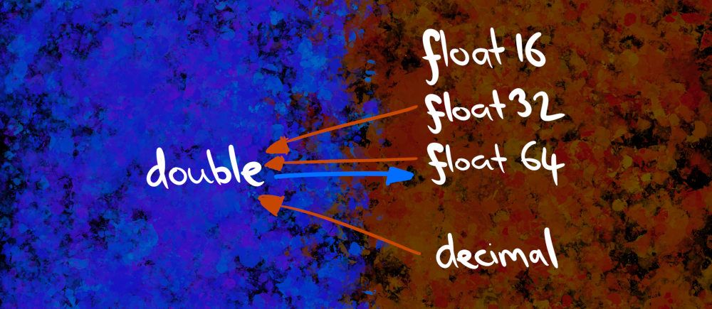
By now you’re probably getting used to the fact that Arrow tends to have more primitive types than R in most situations. Floating point numbers are no exception. R has only a single class, usually referred to as numeric but sometimes called double. In contrast, Arrow has three: float64, float32 and float16.22 It also has another numeric type called decimal that I’ll discuss later.
The easiest of these to discuss is float64, because it adopts the same conventions as the R double class. Just like R, it uses 64 bits to represent a floating point number.23 Because the data structures are so similar, the default behaviour in arrow is to translate an R double into an Arrow float64 and vice versa.
As always, I’ve got a little diagram summarising all the default mappings:
Let’s have a look at the Arrow float64 type. It’s a little anticlimactic in a sense, because it’s the same data structure as the R double type, so all we’re going to “learn” is that it behaves the same way! First, let’s create one:
float_01 <- scalar(0.1)
float_01
Scalar
0.1As always, we’ll verify that the created object has the type we’re expecting…
float_01$typeFloat64
double… and it does, but you might be slightly puzzled by the output this time. What’s going on with the top line and the bottom line? Why does one say “Float64” and the other say “double”?
We’ve seen the “two lines of output” pattern earlier in the post when printing out an int32, but last time the two lines both said the same thing so I didn’t bother to comment on it. This time, however, there’s something to unpack. The distinction here refers to the name of the object type at the R level and and the C++ level. The first line of the output reads “Float64” because that’s what this data structure is called at the R level (i.e., according to arrow). The second line reads “double” because that’s what this data structure is called at the C++ level (i.e., in libarrow). There are a few cases where the arrow package adopts a slightly different naming scheme to libarrow, and so you’ll see this happen from time to time later in the post. There are some good reasons for this difference in nomenclature, and it’s nothing to be concerned about!
Anyway, getting back to the main thread… since we’ve created the value 0.1 as a float64 in Arrow, let’s go through the same exercise we did in R and show that Arrow floats produce the same floating point errors. We’ll create new variables for 0.2 and 0.3:
float_02 <- scalar(0.2)
float_03 <- scalar(0.3)
Just like we saw in R, the logical test of equality gives a counterintuitive answer:
float_01 + float_02 == float_03Scalar
false… and just like we saw in R, the reason for it is that there’s a very small rounding error:
float_01 + float_02 - float_03Scalar
5.551115123125783e-17Just so you don’t have to scroll up to check, yes, the rounding error is the same as the one that R produces:
0.1 + 0.2 - 0.3[1] 5.551115e-17R and Arrow implement the same standard for floating point arithmetic, and so they “fail” in the same way because the failure occurs at the level of the standard. But we don’t blame IEEE 754 for that, because it’s literally impossible to define any standard that will encode the real numbers in an error-free way on a finite-precision machine.
[Arrow] The float32 and float16 types
The float64 type provides an excellent, high precision floating point representation of numeric data. As data types go it is a good type. However, it is a 64-bit type, and sometimes you don’t need to store your data at a high degree of precision. With that in mind, because Arrow places a strong emphasis on both scalability and efficiency, it also provides the float32 type and the float16 type (though float16 hasn’t really been implemented yet, as far as I know). Encoding numeric data in these formats will save space, but will come at a cost of precision. As always, the decision of what encoding works best for your application will depend on what your needs are.
As far as the arrow package is concerned, there are no difficulties in passing data back and forth between R doubles and Arrow float32 types, but at present it’s not really possible to do this with float16 because this isn’t implemented. Still, we can briefly take a look at how it works for float32. Here’s an example of me passing an R double to Arrow:
float32_01 <- scalar(.1, type = float32())
float32_01
Scalar
0.1Let’s quickly verify that it is in fact a 32-bit float:
float32_01$typeFloat32
floatAnd now let’s pull it back into R where it will be, once again, encoded as a double:
as.vector(float32_01)[1] 0.1Yay! It works!
Decimal floating point numbers?
It’s time to talk about decimals. This is a fun topic, but I need to start with a warning: I mentioned that Arrow has a decimal type, and your first instinct as an R programmer might be to assume that this is another variation of floating point numbers. Fight this instinct: it’s not quite right.
Okay, ready?
Earlier in this section I promised that the Baudrillard quote from Simulacra and Simulation was going to be relevant? Well, that time has arrived. It’s also the moment at which the quote from Word and Object by Quine that opened this blog post becomes painfully relevant. Stripped of their fancy language, here’s what the two authors are telling us in these passages:
- The Baudrillard quote emphasises that floating point numbers are a simulation. They are the mechanism by which we pretend to encode real numbers on computers. It’s a lie, but it’s a powerful lie that almost works.
- The Quine quote emphasises that translation (and, I would argue, simulation also) is underdetermined. For any complicated thing there are many ways to simulate, or translate, or approximate it. These approximations can be extremely accurate and still be inconsistent with each other.
Quine’s truism applies to floating point numbers, and it is the reason why “decimal floating point” numbers exist in addition “binary floating point” numbers. All floating point systems are simulations in the Baudrillard sense of the term: lies, strictly speaking, but close enough to true that the distinction between lies and truth gets a little blurry.
Let’s see how that plays out with floating point numbers. When discussing doubles in R, I mentioned that they represent the real numbers using a decomposition that looks like this:
\[ (\mbox{real number}) = (\mbox{sign}) \times (\mbox{mantissa}) \times 2 ^ {\mbox{(exponent)}} \]
The number “2” pops out here, doesn’t it? Is there any reason to think that “2” is a pre-ordained necessity when approximating the real numbers on a finite-precision machine? Programmers have a tendency to like using “2” as the base unit for everything because it lines up nicely with binary representations, and that’s often a good instinct when dealing with machines.
Unfortunately, life consists of more than machines.
In particular, binary representations create problems for floating point arithmetic because the world contains entities known as “humans”, who have a habit of writing numbers in decimal notation24. Numbers that look simple in decimal notation often look complicated in binary notation and vice versa. As we saw earlier, a “simple” decimal number like 0.1 doesn’t have a short binary expansion and so cannot be represented cleanly in a finite-precision binary floating point number system. Rounding errors are introduced every time a machine uses (base 2) floating point to encode data that were originally stored as a (base 10) number in human text.
A natural solution to this is to design floating point data types that use other bases. It is entirely possible to adopt decimal floating point types that are essentially equivalent to the more familiar binary floating point numbers, but they rely on a base 10 decomposition:
\[ (\mbox{real number}) = (\mbox{sign}) \times (\mbox{mantissa}) \times 10 ^ {\mbox{(exponent)}} \]
The virtues of decimal floating point seem enticing, and it’s tempting to think that this must be what Arrow implements. However, as we’ll see in the next section, that’s not true.
Instead of using floating-point decimals, it supplies “fixed-point” decimal types. In a floating-point representation, the exponent is chosen automatically, and it is a property of the value itself. The number -9.832 will always have an exponent of 3 when encoded as a binary floating-point number (as we saw in the polar_g example earlier), and that exponent will never be influenced by the values of other numbers stored in the same data set.
A fixed-point representation is different. The exponent – and in a decimal representation, remember that the exponent is just “the location of the decimal point” – is chosen by the user. You have to specify where the decimal point is located manually, and this location will be applied to each value stored in the object. In other words, the exponent – which is now called the “scale”, and is parameterised slightly differently – becomes a property of the type, not the value.
Sigh. Nothing in life is simple, is it? It’ll become a little clearer in the next section, I promise!
[Arrow] The decimal fixed-point types
Arrow has two decimal types, a decimal128 type that (shockingly) uses 128 bits to store a floating point decimal number, and a decimal256 type that uses 256 bits. As usual arrow package supplies type functions decimal128() and decimal256() that allow you to specify decimal types. Both functions have two arguments that you must supply:
precisionspecifies the number of significant digits to store, similar to setting the length of the mantissa in a floating-point representation.scalespecifies the number of digits that should be stored after the decimal point. If you setscale = 2, exactly two digits will be stored after the decimal point. If you setscale = 0, values will be rounded to the nearest whole number. Negative scales are also permitted (handy when dealing with extremely large numbers), soscale = -2stores the value to the nearest 100.
One convenience that exists both in the arrow R package and within libarrow itself is that it can automatically decide whether you need a decimal128 or a decimal256 simply by looking at the value of the precision argument. If the precision is 38 or less, you can encode the data with a decimal128 type. Larger values require a decimal256. If you would like to take advantage of this – as I will do in this post – you can use the decimal() type function which will automatically create the appropriate type based on the specified precision.
One inconvenience that I have in this post, however, is that R doesn’t have any analog of a fixed-point decimal, and consequently I don’t have any way to create an “R decimal” that I can then import into Arrow. What I’ll do instead is create a floating point array in Arrow, and then explicitly cast it to a decimal type. Step one, create the floating point numbers in Arrow:
floats <- chunked_array(c(.01, .1, 1, 10, 100), type = float32())
floats
ChunkedArray
<float>
[
[
0.01,
0.1,
1,
10,
100
]
]Step two, cast the float32 numbers to decimals:
decimals <- floats$cast(decimal(precision = 5, scale = 2))
decimals
ChunkedArray
<decimal128(5, 2)>
[
[
0.01,
0.10,
1.00,
10.00,
100.00
]
]These two arrays look almost the same (especially because I chose the scale judiciously!), but the underlying encoding is different. The original floats array is a familiar float32 type, but if we have a look at the decimals object we see that it adopts a quite different encoding:
decimals$typeDecimal128Type
decimal128(5, 2)To illustrate that these do behave differently, let’s have fun making floating point numbers misbehave again:
sad_floats <- chunked_array(c(.1, .2, .3))
sum(sad_floats)
Scalar
0.6000000000000001Oh noes. Okay, let’s take a sad float32 and turn it into a happy decimal. I’ll store it as a high precision decimal to make it a little easier to compare the results:
happy_decimals <- sad_floats$cast(decimal(20, 16))Now let’s look at the two sums side by side:
sum(sad_floats)
sum(happy_decimals)
Scalar
0.6000000000000001
Scalar
0.6000000000000000Yay!
As a final note before moving on, it is (of course!!!) the case that fixed-point decimals aren’t a universal solution to the problems of binary floating-point numbers. They have limitations of their own and there are good reasons why floats remain the default numeric type in most languages. But they have their uses: binary and decimal systems provide different ways to simulate the reals, as do fixed and floating point systems. Each such system is a lie, of course: the reals are too big to be captured in any finite system we create. They are, however, useful.

Character types
Our journey continues. We now leave behind the world of number and enter the domain of text. Such times we shall have! What sights we shall see! (And what terrors lie within?)
Strings are an interesting case. R uses a single data type to represent strings (character vectors) but Arrow has two types, known as strings and large_strings. When using the arrow package, Arrow strings are specified using the utf8() function, and large strings correspond to the large_utf8() type. The default mapping is to assume that an R character vector maps onto the Arrow utf8() type, as shown below:

There’s a little more than meets the eye here though, and you might be wondering about the difference between strings and large_strings in Arrow, and when you might prefer one to the other. As you might expect, the large string type is suitable when you’re storing large amounts of text, but to understand it properly I need to talk in more depth about how R and Arrow store strings, and I’ll use this partial list of people that – according to the lyrics of Jung Talent Time by TISM – were perhaps granted slightly more fame than they had earned on merit:
Bert Newton
Billy Ray Cyrus
Warwick Capper
Uri Geller
Samantha Fox
[R] The character class
Suppose I want to store this as a character vector in R, storing only the family names for the sake of brevity and visual clarity.
jung_talent <- c("Newton", "Cyrus", "Capper", "Geller", "Fox")Each element of the jung_talent vector is a variable-length string, and is stored internally by R as an array of individual characters25 So, to a first approximation, your mental model of how R stores the jung_talent variable might look something like this:
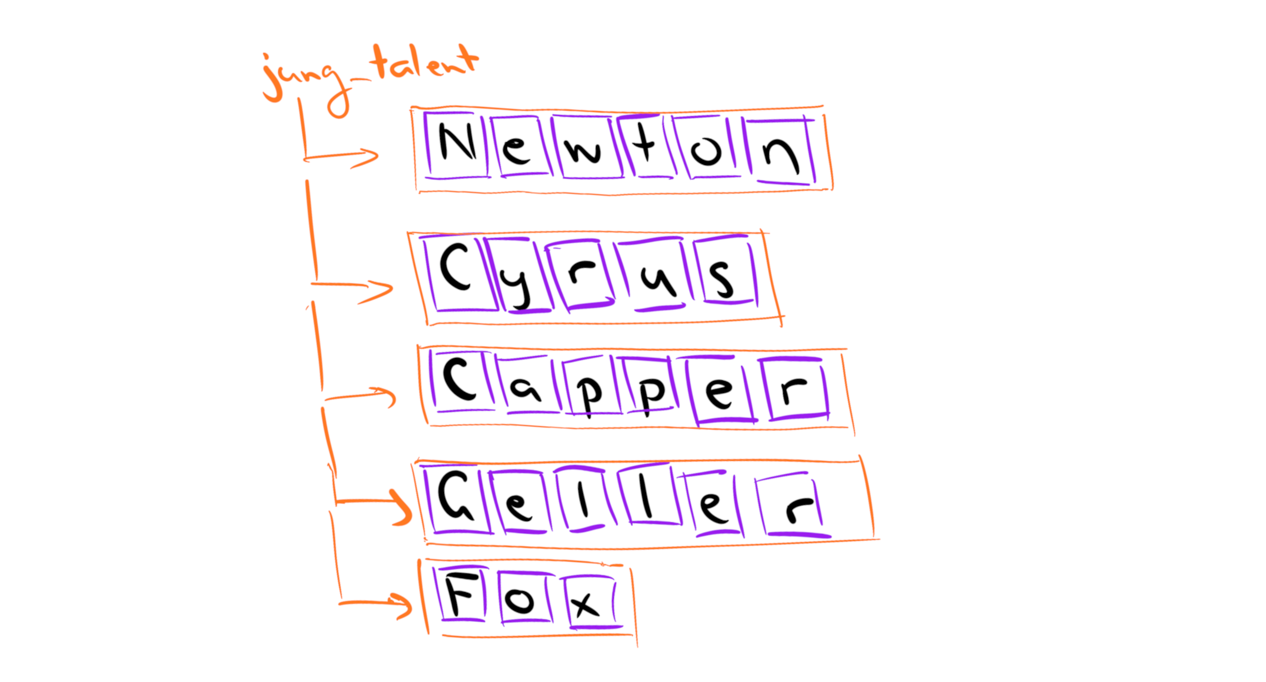
Here, the jung_talent variable is an object26 that contains five elements shown as the orange boxes. Internally, each of those orange boxes is itself an array of individual characters shown as the purple boxes. As a description of what R actually does this is a bit of an oversimplification because it ignores the global string pool, but it will be sufficient for the current purposes.
The key thing to understand conceptually is that R treats the elements of a character vector as the fundamental unit. The jung_talent vector is constructed from five distinct strings, "Newton", "Cyrus", etc. The "Newton" string is assigned to position 1, the "Cyrus" string is assigned to position 2, and so on.
[Arrow] The utf8 type
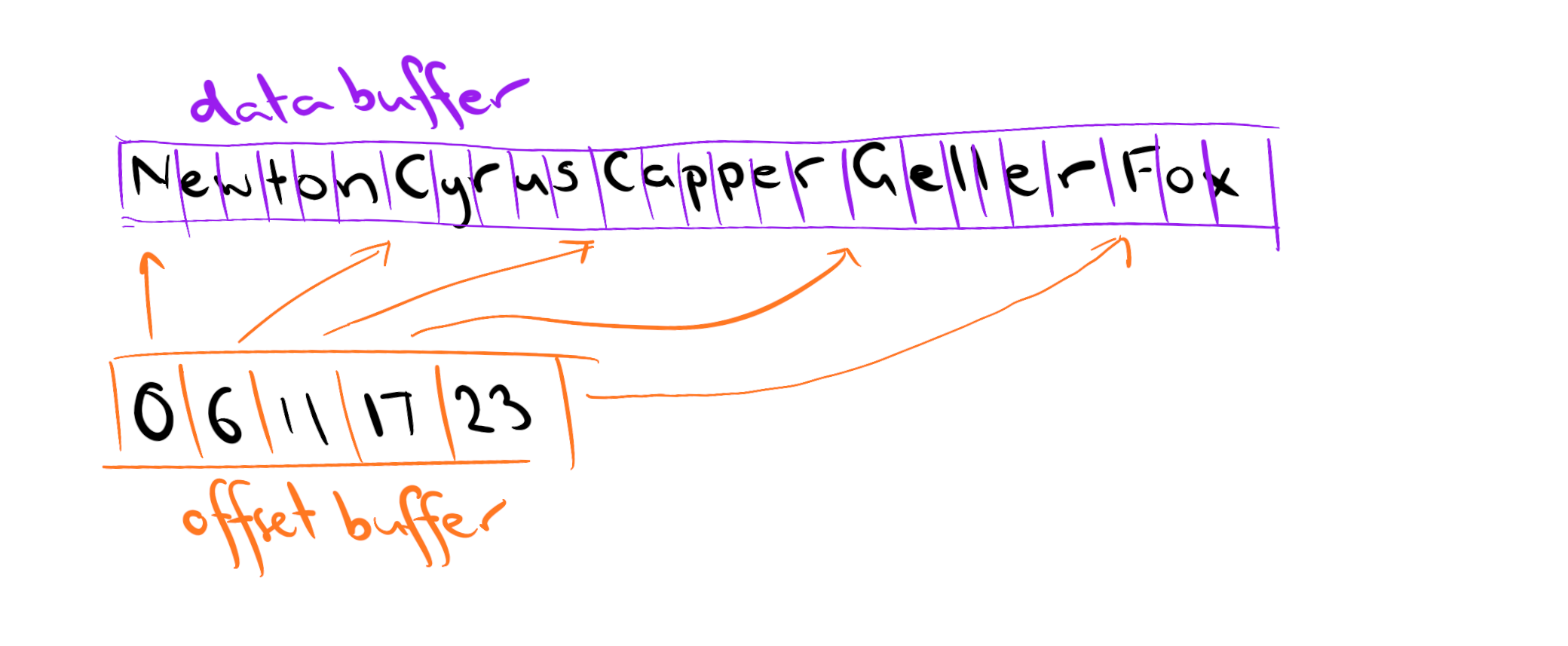
The approach taken in Arrow is rather different. Instead of carving up the character vector into strings (and internally treating the strings as character arrays), it concatenates everything into one long buffer. The text itself is dumped into one long string, like this:
NewtonCyrusCapperGellerFoxThe first element of this buffer – the letter "N" – is stored at “offset 0” (indexing in Arrow starts at 0), the second element is stored at offset 1, and so on. This long array of text is referred to as the “data buffer”, and it does not specify where the boundaries between array elements are. Those are stored separately. If I were to create an Arrow string array called jung_talent_arrow, it would be comprised of a data buffer, and an “offset buffer” that specifies the positions at which each element of the string array begins. In other words, we’d have a mental model that looks a bit like this:
How are each of these buffers encoded?
The contents of the data buffer are stored as UTF-8 text, which is itself a variable length encoding: some characters are encoded using only 8 bits while others require 32 bits. This blog post on unicode is a nice explainer.
The contents of the offset buffer are stored as unsigned integers, either 32 bit or 64 bit, depending on which of the two Arrow string array types you’re using. I’ll unpack this in the next section.
Sheesh. That was long. Let’s give ourselves a small round of applause for surviving, and now actually DO something. We’ll port the jung_talent vector over to Arrow.
jung_talent_arrow <- chunked_array(jung_talent)
jung_talent_arrow
ChunkedArray
<string>
[
[
"Newton",
"Cyrus",
"Capper",
"Geller",
"Fox"
]
]That certainly looks like text to me! Let’s take a look at the data type:
jung_talent_arrow$typeUtf8
stringYep. Definitely text!
[Arrow] The large_utf8 type
Okay, so as I mentioned, Arrow has two different string types: it has strings (also called utf8) and large_strings (also called large_utf8).27 The default in arrow is to translate character data in R to the utf8 data type in Arrow, but we can override this if we want to. In order to help you make an informed choice, I’ll dig a little deeper into the difference between the two types.
The first thing to recognise is that the nature of the data buffer is the same for utf8 and large_utf8: the difference between the two lies in how the offset buffers are encoded. When character data are encoded as utf8 type, every offset value is stored as an unsigned 32-bit integer. That means that – as shown in the table of integer types earlier in the post – you cannot store an offset value larger than 4294967295. This constrain places a practical cap on the total length of the data buffer: if total amount of text stored in the data buffer is greater than about 2GiB, the offset buffer can’t encode the locations within it! Switching to large_utf8 means that the offset buffer will store every offset value as an unsigned 64-bit integer. This means that the offset buffer now takes up twice as much space, but it allows you to encode offset values up to… um… 18446744073709551615. And if you’ve got so much text that your data buffer is going to exceed that limit, well, frankly you have bigger problems.
In short, if you’re not going to exceed 2GiB of text in your array, you don’t need large_utf8. Once you start getting near that limit, you might want to think about switching:
jung_talent_arrow_big <- chunked_array(jung_talent, type = large_utf8())
jung_talent_arrow_big$type
LargeUtf8
large_stringBefore moving on, I’ll mention one additional complexity. This is a situation where the distinction between Arrays and ChunkedArrays begins to matter. Strictly speaking, I lied earlier when I said there’s only one data buffer. A more precise statement would be to say that there is one data buffer per chunk (where each chunk in a ChunkedArray is an Array). ChunkedArrays are designed to allow a block (or “chunk”) of contiguous rows in a table to be stored together in a single location (or file). There are good reasons for doing that28, but they aren’t immediately relevant. What matters is to recognise that in a ChunkedArray, the 2GiB limit on utf8 type data applies on a per-chunk basis. The net result of this is that you probably don’t need large_utf8 except in very specific cases.

Date/time types
Next up on our tour of data types are dates and times. Internally, R and Arrow both adopt the convention of measuring time in terms of the time elapsed since a specific moment in time known as the unix epoch. The unix epoch is the time 00:00:00 UTC on 1 January 1970. It was a Thursday.
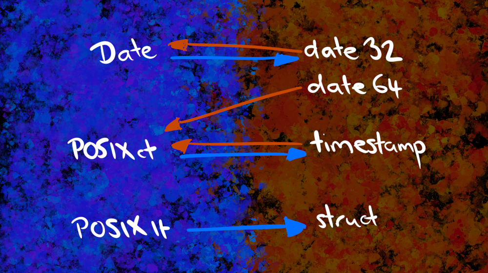
Despite agreeing on fundamentals, there are some oddities in the particulars. Base R has three date/time classes (Date, POSIXct, and POSIXlt), and while Arrow also has three date/time classes (date32, date64, and timestamp), the default mappings between them are a little puzzling unless you are deeply familiar with what all these data types are and what they represent. I’ll do the deep dive in a moment, but to give you the big picture here’s how the mapping works:
[R] The Date class
On the R side of things, a Date object is represented internally as a numeric value, counting the number of days since the unix epoch. Here is today as a Date:
today <- Sys.Date()
today
[1] "2023-05-27"If I use unclass() to see what it looks like under the hood:
unclass(today)[1] 19504Fundamentally, a Date object is a number:29 it counts the number of days that have elapsed since a fixed date. It does not care what the year is, what the month is, or what day of the month it is. It does not care how the date is displayed to the user. All those things are supplied by the print() method, and are not part of the Date itself.
[R] The POSIXct class
A date is a comparatively simple thing. When we want to represent dates and time together, we need to know the time of day, and we might need to store information about the timezone as well (more on that later). Base R has two different classes for representing this, POSIXct and POSIXlt. These names used to confuse me a lot. POSIX stands for “portable operating system interface”, and it’s a set of standards used to help operating systems remain compatible with each other. In this context though, it’s not very meaningful: all it says “yup we use unix time.”
The more important part of the name is actually the “ct” versus “lt” part. Let’s start with POSIXct. The “ct” in POSIXct stands for “calendar time”: internally, R stores the number of seconds30 that have elapsed since 1970-01-01 00:00 UTC.
now <- Sys.time()
now
[1] "2023-05-27 18:24:15 AEST"If I peek under the hood using unclass() here’s what I see:
unclass(now)[1] 1685175855There are no attributes attached to this object, it is simply a count of the number of seconds since that particular moment in time. However, it doesn’t necessarily have to be this way: a POSIXct object is permitted to have a “tzone” attribute, a character string that specifies the timezone that is used when printing the object will be preserved when it is converted to a POSIXlt.
Nevertheless, when I created the now object by calling Sys.time(), no timezone information was stored in the object. The fact that it appears when I print out now occurs because the print() method for POSIXct objects prints the time with respect to a particular timezone. The default is to use the system timezone, which you can check by calling Sys.timezone(), but you can override this behaviour by specifying the timezone explicitly (for a list of timezone names, see OlsonNames()). So if I wanted to print the time in Berlin, I could do this:
print(now, tz = "Europe/Berlin")[1] "2023-05-27 10:24:15 CEST"If you want to record the timezone as part of your POSIXct object rather than relying on the print method to do the work, you can do so by setting the tzone attribute. To illustrate this, let’s pretend I’m in Tokyo:
attr(now, "tzone") <- "Asia/Tokyo"
now
[1] "2023-05-27 17:24:15 JST"The important thing here is that the timezone is metadata used to change the how the time is displayed. Changing the timezone does not alter the number of seconds stored in the now object:
unclass(now)[1] 1685175855
attr(,"tzone")
[1] "Asia/Tokyo"[R] The POSIXlt class
What about POSIXlt? It turns out that this is a quite different kind of data structure, and it “thinks” about time in a very different way. The “lt” in POSIXlt stands for “local time”, and internally a POSIXlt object is a list that stores information about the time in a way that more closely mirrors how humans think about it. Here’s what now looks like when I coerce it to a POSIXlt object:
now_lt <- as.POSIXlt(now)
now_lt
[1] "2023-05-27 17:24:15 JST"It looks exactly the same, but this is an illusion produced by the print() method. Internally, the now_lt object is a very different kind of thing. To see this, let’s see what happens if we print it as if it were a regular list:
unclass(now_lt)$sec
[1] 15.1697
$min
[1] 24
$hour
[1] 17
$mday
[1] 27
$mon
[1] 4
$year
[1] 123
$wday
[1] 6
$yday
[1] 146
$isdst
[1] 0
$zone
[1] "JST"
$gmtoff
[1] 32400
attr(,"tzone")
[1] "Asia/Tokyo" "JST" "JDT"
attr(,"balanced")
[1] TRUEAs you can see, this object separately stores the year (counted from 1900), the month (where January is month 0 and December is month 11), the day of the month (starting at day 1), etc.31 The timezone is stored, as is the day of the week (Sunday is day 0), it specifies whether daylight savings time is in effect, and so on. Time, as represented in the POSIXlt class, uses a collection of categories that are approximately the same as those that humans use when we talk about time.
It is not a compact representation, and it’s useful for quite different things than POSIXct. What matters for the current purposes is that POSIXlt is, fundamentally, a list structure, and is not in any sense a “timestamp”.
[Arrow] The date32 type
Okay, now let’s pivot over to the Arrow side and see what we have to work with. The date32 type is similar – but not identical – to the R Date class. Just like the R Date class, it counts the number of days since 1970-01-01. To see this, let’s create an analog of the today Date object inside Arrow, and represent it as a date32 type:
today_date32 <- scalar(today, type = date32())
today_date32
Scalar
2023-05-27We can expose the internal structure of this object by casting it to an int32:
today_date32$cast(int32())Scalar
19504This is the same answer we got earlier when I used unclass() to take a peek at the internals of the today object. That being said, there is a subtle difference: in Arrow, the date32 type is explicitly a 32-bit integer. If you read through the help documentation for date/time classes in R you’ll see that R has something a little more complicated going on. The details don’t matter for this post, but you should be aware that Dates (and POSIXct objects) are stored as doubles. They aren’t stored as integers:
typeof(today)
typeof(now)[1] "double"
[1] "double"In any case, given that the Arrow date32 type and the R Date class are so similar to each other in structure and intended usage, it is natural to map R Dates to Arrow date32 types and vice versa, and that’s what the arrow package does by default.
[Arrow] The date64 type
The date64 type is similar to the date32 type, but instead of storing the number of days since 1970-01-01 as a 32-bit integer, it stores the number of milliseconds since 1970-01-01 00:00:00 UTC as a 64-bit integer. It’s similar to the POSIXct class in R, except that (1) it uses milliseconds instead of seconds; (2) the internal storage is an int64, not a double; and (3) it does not have metadata and cannot represent timezones.
As you might have guessed, the date64 type in Arrow isn’t very similar to the Date class in R. Because it represents time at the millisecond level, the intended use of the date64 class is in situations where you want to keep track of units of time smaller than one day. Sure, I CAN create date64 objects from R Date objects if I want to…
scalar(today, date64())Scalar
2023-05-27…but this is quite wasteful. Why use a 64-bit representation that tracks time at the millisecond level when all I’m doing is storing the date? Although POSIXct and date64 aren’t exact matches, they’re more closely related to each other than Date and date64. So let’s create an Arrow analog of now as a date64 object:
now_date64 <- scalar(now, date64())
now_date64Scalar
2023-05-27The output is printed as a date, but this is a little bit misleading because it doesn’t give you a good sense of the level of precision in the data. Again we can peek under the hood by explicitly casting this to a 64-bit integer:
now_date64$cast(int64())Scalar
1685175855169This isn’t a count of the number of days since the unix epoch, it’s a count of the number of milliseconds. It is essentially the same number, divided by 1000, as the one we obtained when I typed unclass(now).
However, there’s a puzzle here that we need to solve. Let’s take another look at unclass(now):
unclass(now)[1] 1685175855
attr(,"tzone")
[1] "Asia/Tokyo"This might strike you as very weird. On the face of it, what has happened is that I have taken now (which ostensibly represents time at “second-level” precision), ported it over to Arrow, and created an object now_date64 that apparently knows what millisecond it is???? How is that possible? Does Arrow have magic powers?
Not really. R is playing tricks here. Remember how I said that POSIXct objects are secretly doubles and not integers? Well, this is where that becomes relevant. It’s quite hard to get R to confess that a POSIXct object actually knows the time at a more precise level than “to the nearest second” but you can get it do to so by coercing it to a POSIXlt object and then taking a peek at the sec variable:
as.POSIXlt(now)$sec[1] 15.1697Aha! The first few digits of the decimal expansion are the same ones stored as the least significant digits in now_date64. The data was there all along. Even though unclass(now) produces an output that has been rounded to the nearest second, the original now variable is indeed a double, and it does store the time a higher precision! Ultimately, the accuracy of the time depends on the system clock itself, but the key thing to know here is that even though POSIXct times are almost always displayed to the nearest second, they do have the ability to represent more precise times.
Because of this, the default behaviour in arrow is to convert date64 types (64-bit integers interpreted as counts of milliseconds) to POSIXct classes (which are secretly 64-bit doubles interpreted as counts of seconds).
Right. Moving on.
[Arrow] The timestamp type
The last of the Arrow date/time types is the timestamp. The core data structure is a 64-bit integer used to count the number of time units that have passed since the unix epoch, and this is associated with two additional pieces of metadata: the time unit used (e.g., “seconds”, “milliseconds,”microseconds”, “nanoseconds”), and the timezone. As with the POSIXct class in R, the timezone metadata is optional, but the time unit is necessary. The default is to use microseconds (i.e., unit = "us"):
scalar(now)
scalar(now, timestamp(unit = "us"))Scalar
2023-05-27 08:24:15.169700
Scalar
2023-05-27 08:24:15.169700Alternatively, we could use seconds:
scalar(now, timestamp(unit = "s"))Scalar
2023-05-27 08:24:15It’s important to recognise that changing the unit does more than change the precision at which the timestamp is printed. It changes “the thing that is counted”, so the numbers that get stored in the timestamp are quite different depending on the unit. Compare the numbers that are stored when the units are seconds versus when the units are nanoseconds:
scalar(now, timestamp(unit = "s"))$cast(int64())
scalar(now, timestamp(unit = "ns"))$cast(int64())Scalar
1685175855
Scalar
1685175855169700864Okay, what about timezone?
Recall that now has a timezone attached to it, because I explicitly recorded the tzone attribute earlier. Admittedly I lied and I said I was in Tokyo and not in Sydney, but still, that information is in the now object:
now[1] "2023-05-27 17:24:15 JST"When I print the R object it displays the time in the relevant time zone. The output for the Arrow object doesn’t do that: the time as displayed is shown in UTC. However, that doesn’t mean that the metadata isn’t there:
now_timestamp <- scalar(now)
now_timestamp$type
Timestamp
timestamp[us, tz=Asia/Tokyo]I mention this because this caused me a considerable amount of panic at one point when I thought my timezone information had been lost when importing data from POSIXct into Arrow. Nothing was lost, it is simply that the arrow R package prints all timestamps in the corresponding UTC time regardless of what timezone is specified in the metadata.
There is, however, a catch. This worked last time because I was diligent and ensured that my now variable encoded the timezone. By default, a POSIXct object created by Sys.time() will not include the timezone. It’s easy to forget this because the print() method for POSIXct objects will inspect the system timezone if the POSIXct object doesn’t contain any timezone information, so it can often look like you have a timezone stored in your POSIXct object when actually you don’t. When that happens, Arrow can’t help you. Because the POSIXct object does not have a timezone (all appearances to the contrary), the object that arrives in Arrow won’t have a timezone either. Here’s what I mean:
# a POSIXct object with no timezone
new_now <- Sys.time() # has no time zone...
new_now               # ... but appears to!
[1] "2023-05-27 18:24:15 AEST"# an Arrow timestamp with no timezone
new_now_timestamp <- scalar(new_now)
new_now_timestamp$typeTimestamp
timestamp[us, tz=Australia/Sydney]The take-home message in all this is that if you’re going to be working in both Arrow and R, and using the arrow package for data interchange, you’d be well advised to be careful with your POSIXct objects and timezones. They are trickier than they look, and can lead to subtle translation errors if you are not careful!
Um, but what about POSIXlt?
At long last we come to POSIXlt, which has no clear analog in Arrow. The key idea behind POSIXlt is to represent temporal information in terms of multiple different units: days, weeks, years, seconds, timezones, and so on. It’s a very different kind of thing to a POSIXct object in R or a timestamp in Arrow. In R terms, it’s essentially a list, and as a consequence the default behaviour in arrow is to import it as a struct (which serves essentially the same purpose). Here’s how that looks:
scalar(now_lt)Scalar
2023-05-27 17:24:15The struct object contains named fields that are identical to their POSIXlt equivalents, and whose types have been translated according to the default mappings: sec is a double, min is an int32, hour is an int32, zone is a string, and so on.
This arrangement, where POSIXct maps to timestamp and POSIXlt maps to struct, makes perfect sense when you think about the underlying data structures that POSIXct and POSIXlt encode. Where things can be tricky for the R user is in the “mental account keeping”. In order to be helpful, R displays POSIXct and POSIXlt objects in exactly the same way:
now
now_lt
[1] "2023-05-27 17:24:15 JST"
[1] "2023-05-27 17:24:15 JST"Not only that, because POSIXct and POSIXlt are both subclasses of the POSIXt class, R allows you to perform temporal arithmetic on objects of different types:
now - now_ltTime difference of 0 secsThis is very convenient from a data analysis perspective, since calculations performed with date/time classes “just work” even though POSIXct objects are secretly doubles and POSIXlt objects are secretly lists. However, all this happens invisibly. In much the same way that it’s easy to forget that POSIXct objects may not encode a timezone even though they look like they do, it can be easy to forget that POSIXct and POSIXlt are fundamentally different objects, and they map onto quite different data structures in Arrow.

Duration types
Any discussion of temporal data is incomplete without a discussion of duration types, which are used to describe a length of time without reference to any fixed origin. The figure below shows the default mappings used by arrow:
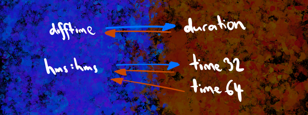
[R] The difftime class
In base R, the difference between two date/time objects is stored as a difftime object. To give a better illustration of a difftime object, let’s create diff, a variable that stores the amount of time elapsed between executing the R markdown chunk that first computed the now variable, and executing the R markdown chunk below:
new_now <- Sys.time()
rmd_time <- new_now - now
rmd_time
Time difference of 0.3497994 secsNow let’s take a look at how it’s actually stored:
unclass(rmd_time)[1] 0.3497994
attr(,"units")
[1] "secs"The duration is represented as a double variable, and the "units" attribute is used to specify the time unit that it represents: “secs”, “mins”, “hours”, “days” or “weeks”. Unless the user specifies exactly which unit is to be used, R will attempt to make a sensible choice. For instance, if I were to do this,
hedy_lamarr <- as.POSIXct("1914-11-09 19:30:00", tz = "Europe/Vienna")
hedy_age <- now - hedy_lamarr
hedy_age
Time difference of 39645.58 daysI would learn that it has been 39646 days since Hedy Lamarr was born.32 More to the point, R has guessed that the length of time is sufficiently long that “seconds” aren’t the appropriate encoding unit:
unclass(hedy_age)[1] 39645.58
attr(,"units")
[1] "days"[Arrow] The duration type
The difftime class in R has a natural analog in Arrow, the duration type. As usual though, they are not exactly equivalent to one another. An R difftime object stores the value as a double, so it has no problems storing 0.35 as the value and setting the units to be seconds. This doesn’t work very well in Arrow because the value is stored as a signed 64 bit integer (int64), and a value of 0.35 seconds will simply round down to a duration of zero seconds. When importing my duration data into Arrow, then, I should be careful to ensure I choose a higher precision unit. If I don’t, things can go a little awry:
rmd_time_arrow <- scalar(rmd_time)
rmd_time_arrow
Scalar
0Hm. Zero seconds was not exactly the answer I was looking for. It helps a little to take a peek at the data type and see what precisely it is that I have just created:
rmd_time_arrow$typeDurationType
duration[s]This reveals my mistake. I’ve encoded the time rounded to the nearest second, which is not very useful in this instance. What I really should have done is specify a higher level of precision. To import a duration into Arrow rounded to the nearest microsecond, I can do this:
rmd_time_arrow <- scalar(rmd_time, duration(unit = "us"))
rmd_time_arrow
Scalar
349799That’s a little better! Again, I can inspect the data type and see that the unit of encoding is now set to microseconds:
rmd_time_arrow$typeDurationType
duration[us][R] The hms::hms class
So where are we up to in our voyage through the world of dates, times, and durations in the R world? We’ve talked about situations where you can specify a fixed date (with the Date class) and situations where you can specify a fixed moment in time (with POSIXct and POSIXlt classes). We’ve also talked about situations where you can specify an amount of time without fixing it to a specific date or time (with the difftime class). What we haven’t talked about is how to store the time of day. In base R you can talk about a date without needing to specify a time, or you can talk about times and dates together, but what you can’t do is specify a time on its own without a date.
The hms package fixes this by supplying the hms class. Internally, it’s just a difftime object that counts the number of seconds elapsed since midnight. As I type these words the current time is 14:05:25, and I could create an hms object representing this like so:
hms_time <- hms::hms(seconds = 25, minutes = 5, hours = 14)
hms_time14:05:25The nice thing about hms times is that they inherit from difftime, which we can see by checking the class vector for our hms_time object
class(hms_time)[1] "hms" "difftime"Just to show that there really isn’t anything fancy going on, let’s strip the class attribute away and let R print out the raw object. As the output here shows, an hms object has the same underlying structure as a regular difftime object:
unclass(hms_time)[1] 50725
attr(,"units")
[1] "secs"[Arrow] The time32 and time64 types
What about Arrow?
At a technical level, it would be perfectly possible to translate an hms object in R into an Arrow duration object, but that feels slightly unnatural. The entire reason why the hms class exists in R is that we – the human users – attach special meaning to the “duration of time that has elapsed since midnight on an arbitrary day”. We call it the time of day, and while technically it is possible to represent the time of day as a duration (or an hms as a difftime), human beings like to treat special things as special for a reason.
Because of this, Arrow supplies two data types that are roughly analogous to the hms class in R, called time32 and time64. The time32 type stores the time of day as a signed 32-bit integer, which represents the number of seconds (or alternatively, milliseconds) since midnight. By default, the arrow package will translate an hms object to a time32 type, using seconds as the unit:
hms_time32_s <- scalar(hms_time)
hms_time32_s
Scalar
14:05:25As usual, let’s just verify that the encoding unit is as expected:
hms_time32_s$typeTime32
time32[s]Yep, we’re all good! To switch to milliseconds, I would use a command like this:
hms_time32_ms <- scalar(hms_time, time32(unit = "ms"))
hms_time32_ms
Scalar
14:05:25.000Notice that the output shows the time in a little more resolution. I find this a helpful touch, since it provides a visual cue letting me know what the unit is. But just to confirm, let’s inspect the type explicitly:
hms_time32_ms$typeTime32
time32[ms]If you need to represent the time of day at a higher degree of precision, you’ll want to use the time64 type, which (shockingly!) represents the time of day as a signed 64-bit integer. When using the time64 class you can choose microseconds (unit = "us") or nanoseconds (the default, unit = "ns") as the unit:
hms_time64_us <- scalar(hms_time, time64())
hms_time64_us
Scalar
14:05:25.000000000The display is showing more trailing zeros, so you can already be sure that the encoding unit has changed. So the only real question you might have pertains to the author. Will she be tediously predictable and check the data type yet again to verify that the encoding unit is nanoseconds, just like she has done every time before? Yes. Yes she will:
hms_time64_us$typeTime64
time64[ns]She is quite tiresome at times.
In essence, the arrow defaults are set up such that if you choose time32() when going from R to Arrow without specifying a unit, you will end up with the lowest precision representation of time (rounded to the nearest second), whereas if you do the same with time64() you end up with the highest precision (nanosecond level) representation. When going the other way, arrow will map time32 types and time64 types to hms objects, and the end result is that the time of day will be stored as a double.

Other types
As with any story told by humans, this one is incomplete. When I started writing this post I had the ambition to cover every single line in the Table of R/Arrow mappings shown in the arrow documentation. I didn’t quite get there in the end, and there are a few missing cases. I’ll briefly mention them here:
Arrow possesses a “null” value used to represent missing data, and behaves similarly to
NAin R. In base R there are several differentNAvalues, corresponding to the different atomic types:NA_logical,NA_character. The way this is handled in arrow is to rely on the vctrs package. Specifically, in vctrs there is a vctrs_unspecified class that works very well here, so Arrow nulls map to vctrs_unspecified and vice versa. In practice, this is whereNAvalues enter into the picture.In R there is the concept of the raw type used to represent bytes. Arrow doesn’t have a natural equivalent of this, but the closest is an unsigned 8-bit integer, so the default is to map raw to uint8.
I haven’t talked about factors at all, and frankly I probably should have. My only excuse is exhaustion. The post was getting very long and I ran out of energy. The analog of factors in Arrow is the dictionary type. They’re not exact mirrors of each other so it’s worth reading the documentation, but it’s close enough that factors are mapped to dictionaries and vice versa.
R and Arrow both allow more complicated data structures to be included as columns within a data frame (or Table). For example, in R each element of a column can itself be a data frame. In such cases, the default in arrow is to map each R data frame onto an Arrow struct. Again, this is one where it’s worth reading the documentation, because there are some subtleties with how things like list columns are handled.

The magic goes away
“Being in love ruins my judgement. It takes my mind off what I’m doing, and I ruin spells”
– Mirandee, from The Magic Goes Away by Larry Niven
When I first started using arrow, it was the magic I loved most. Everything just worked. I could move data between R and Arrow without having to think, I could manipulate enormous data sets using dplyr syntax that I’d never even be able to load into R, and I never had to look under the hood. Magic is always compelling. It is delightful. It makes the user feel joy, and it’s the experience the developer wants to provide.
But as any teacher will tell you, the magic always goes away. There comes a time when you have to sit down and read the manuals. You have to understand how the magic works, and when you do understand you realise there is no magic. At best, there is design. A system can work using all the default settings because it has been thoughtfully designed, but you will eventually encounter situations when the defaults don’t apply to you. It’s taken me some time to piece all this together, and at the end of the process I feel a lot more confident in my judgment. Having a deeper understanding of data types in Arrow and R is useful to me, even if I’m only using the default schemas.
I hope the post is helpful for anyone else following a similar path.33
Footnotes
To be honest, if my goal had been to read the data into Arrow, there was never a need to read it into R in the first place. The code
read_csv_arrow("magicians.csv", as_data_frame = FALSE)would create the Table object directly with no need for an intermediary in R. However, for the purposes of this post I’m pretending that I have data in R that I want to transfer to Arrow in order to talk about the translation process, so I’m doing things in a rather inefficient way. On top of that, there’s a whole extra layer of complexity I’m hiding here that relates to ALTREP vectors backed by Arrow. However, that’s a topic for a future post. We can only unravel the magical cloak one thread at a time!↩︎Early in the writing process for this post I talked to the very lovely Jon Keane about this, and they pointed out that there’s a big difference in the “read” functions in arrow and the “translate” functions. The code in the
read_*()functions is complicated: it handles everything for you because “reading the data” is a constrained task and the developers can optimise almost everything for you, including the strange edge cases. Translation is harder, and there’s less the developers can do to support it. As a consequence, the code underpinningschema()is much simpler. It takes care of choices for you when those choices are “obvious”, but it leaves all the edge cases for you to deal with. There are a lot of weird edge cases because “translating between languages” is under-determined. Edge cases are left to the user because only the user knows the context.↩︎If you have never watched The Magicians I really need to emphasise that it was a really, really weird show and this is nowhere near as implausible as it might sound. I have literally scared off men who had previously been quite keen on me by making them watch this show. Not kidding.↩︎
Back my former life as an mathematical psychologist I studied this stuff for a living, and wrote an absurd number of academic papers on how people learn and represent categories. What I wanted to understand was the relationship between human and machine learning, between natural and artificial intelligence, and so on. What I actually learned is that humans and machines are both super weird.↩︎
At this point I feel compelled to point out that while I may appear to be a bright young thing with little experience of the world, I am in fact a 44 year old woman and former academic who has read quite a few papers on algorithmic information theory and related fields. So, if you happen to be thinking thoughts along the lines of “aha, she doesn’t know about Turing equivalence!” and are considering explaining it to me… please don’t. This is one of those situations where that pesky little “finite length” prefix code required to allow machine P to simulate machine Q actually matters, and sometimes “finite” includes values like “staggeringly, painfully large”. As I used to wearily tell my students, in real life you can’t ignore the \(O(1)\) terms.↩︎
As an aside, Michel Foucault actually refers to this Borges passage in the preface to his famous work The Order of Things: An Archaeology of the Human Sciences on how different cultures and historical periods viewed the world from fundamentally different perspectives. According to Foucault, Borges essay “shattered … all the familiar landmarks of thought — our thought, the thought that bears the stamp of our age and our geography — breaking up all the ordered surfaces and all the planes with which we are accustomed to tame the wild profusion of existing things”. Seems fair to say that Borges’ essay was not without its admirers.↩︎
Much like the Honourable Member for Kennedy, this “let a thousand OOP systems bloom” philosophy has made me cry many times: sometimes from joy, often from frustration.↩︎
The typographical notation for R6 varies because the term can be used to refer to the OOP system itself (which I denote as R6), but could also refer to the R6 package or the R6 object type.↩︎
Note that the
Tableobject is not a Table: it is the class prototype for Table objects, and is therefore classed R6ClassGenerator. The same is true forScalar,Schema,ChunkedArray, etc.↩︎Should I take this opportunity to discuss the fact that this means that what R actually implements is a three valued logic? No. No I should not. I am going to think it very loudly though.↩︎
Lest anyone think I am too wanton in my use of footnotes in tech blogging, I will simply mention that Dan has a 77-footnote blog post on Gaussian Processes. I am the nice queer in the room.↩︎
There is also an R6 method you could use here.
snowpiercer$as_vector()would produce exactly the same answer.↩︎Okay that was a tortured metaphor and one that I probably don’t want to push too far given that Snowpiercer is a terrifyingly dark show filled with horrible, horrible people. But I’m nice though. Honest! Would I lie to you?↩︎
Rest assured, dear reader, while I am entirely aware of the distinction between countably and uncountably infinite sets, and have been forced to learn more about the cardinality of transfinite numbers than any human deserves to endure, I will not be discussing any of that in this post. The word “infinite” is perfectly serviceable for our purposes, and if anyone even TRIES to discuss this with me further on twitter I will be forced to engage the services of a very unpleasant lawyer…↩︎
The “desert of the real” phrase in the title of the section refers to the real numbers, but it’s also a quote from Simulacra and Simulation and The Matrix. Obviously I encountered it in The Matrix first because, all appearances to the contrary, I am uncultured swine.↩︎
At this point it is traditional to make a joke about Zeno’s paradox of Achilles and the Tortoise and honestly I did try, but to come up with a good joke I first had to get half an idea, and then I had to refine it half way to being a better idea, and then I had to refine that half way and… I guess I never quite got there in the end. Sorry.↩︎
Sigh. Technically, this is the last bit. R uses a little-endian representation here which I have flipped to a big-endian format so that it can be read from left to right, but for the love of all that is good and precious in this world please let me simplify a few things okay?↩︎
Okay, if you were reading closely earlier you might be thinking this is wrong and the range should be -1023 to 1024. The reason it’s not is that those to values are reserved for “special” numbers.↩︎
I still think “Man Tissa” would make a good drag king name, though I’ve been unreliably informed that it may sound odd to Norwegians.↩︎
In fact, one of the obnoxious things about the reals (which are uncountably infinite) is that almost all reals have infinitely long mantissas. Even if you had a infinite number of digits to work with (a countably infinite set) you’re still in trouble. Everything sucks, real numbers are almost surely uncomputable (yes that’s an actual result), and I don’t want to think about it any more and I need a lie down.↩︎
Okay, so contrary to my stated intentions we’ve actually ended up quite a long way down into the IEEE 754 standard, so I might as well make an extra observation while we’re down here. Tests of floating point equality aren’t tests of mathematical equality. They’re really just checks that the absolute difference between two numbers is smaller than the machine precision. The value of the machine precision is stored in R as
.Machine$double.eps.↩︎Some precision is needed here: in this post I am using the names that appear in the documentation to the arrow R package. I’m doing this because the intended audience is an R user who wants to use the arrow package to interact with Arrow. However, you should be aware that these types are given slightly different names in the C++ documentation to libarrow to which arrow provides bindings. In that documentation the terminology is as follows: float64 is called double, float32 is called float, and float16 is called half-float.↩︎
They are both little-endian too.↩︎
That’s assuming we’re writing numbers in Arabic number system. I suppose it would be different if our orthographic representations adopted the Sumerian sexagesimal notation. Admittedly, neither R nor Arrow existed at the time, so it’s a moot point. All I’m really saying is that decimal systems are no less arbitrary than binary ones. The problem arises because of the mismatch, not because one encoding is inherently better than the other.↩︎
As noted in the R internals manual, the specific data structure is referred to as a CHARSXP. For the purposes of the current post I’m pretending that character strings are always encoded as UTF-8 because there’s no need to complicate matters by talking about things like Latin-1, but be aware that R does support those things. If you’re looking for a good overview of what UTF-8 encoding is all about, this blog post on how unicode works is helpful.↩︎
More strictly, it is a symbol that points to an object. R makes a distinction between the symbol and the object to which it links, and allows multiple labels to point at the same object. There’s an excellent discussion of this in Chapter 3 of Advanced R↩︎
Once again, there’s a little terminology to explain because there’s some inconsistency in how the types are referred to in the Arrow C++ documentation and the arrow R package documentation. In the list of data types for libarrow you’ll find references to string types and large_string types. However, in list of data types documentation for the arrow R package you’ll see the same data types referred to as utf8 and large_utf8.↩︎
No I am not going to talk about them in this post. Masochist though I may be, nobody loves that much pain. If you are curious you will simply have to wait for a later post!↩︎
Perhaps surprisingly, this number is encoded as a double and not an integer.↩︎
Again, this is stored as a double and not an integer. You can verify this with the command
typeof(Sys.time())↩︎A little counterintuitively, the value of
secranges from 0 to 61, presumably because leap seconds are a thing. I am NOT going to torture myself with that one today. My life has quite enough torture in it already.↩︎Yes, I looked up her time and location of birth on an astrology website. I am, after all, a queer. I feel that I have been quite clear on this, and being weird about astrology it is one of the fine traditions of our people.↩︎
A thank you to Jon Keane, Steph Hazlitt, and Neal Richardson for helpful conversations, encouragement, and feedback that have greatly improved the post.↩︎
Reuse
Citation
BibTeX citation:
@online{navarro2022,
  author = {Navarro, Danielle},
  title = {Data Types in {Arrow} and {R}},
  date = {2022-03-04},
  url = {https://blog.djnavarro.net/data-types-in-arrow-and-r},
  langid = {en}
}
For attribution, please cite this work as: